20_00_Problems

Problem solving

Below is a list of the most common problems that occur in various calculations of pipelines and other aspects of working with the Hydrosystem, and ways to solve them (with links to relevant sections of the help system that explain how to get around these problems).

The dongle is not found, a license has not been obtained, etc.

If you receive any messages related to licenses and keys when launching the program, first of all you should check the availability of the key (dongle). If a local usb-dongle is used, it must be connected to the computer on which the Hydrosystem is running; if the network dongle is used, then it must be installed on a computer (server) that can be accessed over the network from the computer on which the Hydrosystem is running. In addition, check whether the dongle drivers are installed and whether access to the dongle is configured correctly - for more information, see here.

If the error "The program was not found in the dongle" (or similar) is returned, make sure that you are using the correct dongle, which contains the license for the Hydrosystem. If the error "the version number does not match" (or similar) is returned, it most likely means that the version of the Hydrosystem you installed is newer than the one specified in your protection dongle which means that you need to update your dongle to use this version. For information on this, see here.

What's my Hydrosystem version number/which versions are available to me

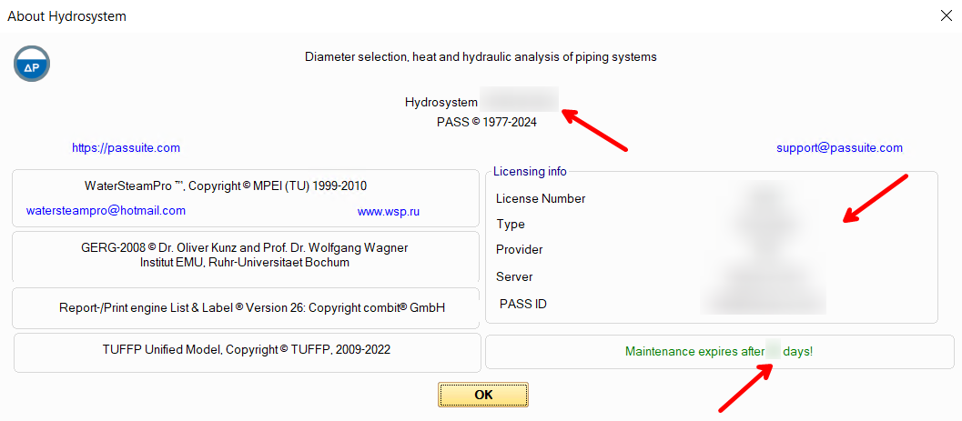
The number of the installed version of the Hydrosystem can be viewed by selecting the menu item "Help - About Hydrosystem..." (there you can also view information about the program maintenance status):

The version history of the program with release dates of all versions and releases can be downloaded here. If you have a valid maintenance for the program, all versions are available for you, including the latest one, which is usually the most recommended for use. If your maintenance period has expired, find your letter of grant for the program (see below) and look at the expiration date of warranty support in it. Then, in the version history, find the version number (namely the version, not the release) that was released last before that date - this version and all its releases (even those that were released after your maintenance period was over) are available to you.

Please note that the security dongle for the program allows to work not with just one specific version number, but with a range of various versions. Therefore, if, for example, for some reason you need to go back to the previous version of the Hydrosystem that you used earlier, you can install it - it will work with your dongle. If the error "the version number does not match" (or similar) is displayed when starting the program, it most likely means that the version of the Hydrosystem you installed is newer than the one specified in your protection dongle. If you are sure that this version is available to you according to the warranty service, you just need to update the information (about the version number of the program) in your protection dongle. The dongle is updated remotely and it requires a minimum of time and effort. All you need to do is save the dongle status bar (for more information, see here) and send it to the organization through which you purchased the Hydrosystem license. In response, you will receive an update string that you will need to upload to the dongle, after which the new version of the program will work with this dongle.

''The license for this type of calculation is not available'' message when running calculation

In this case, first of all, you should check which configuration of the program is purchased in your organization. This information can be found in the Letter of Grant for the program, which is issued upon purchase of the license. It usually looks something like this:

It is possible that you do not have a configuration or module required for the calculation you tried to perform, and you need to purchase it (to do this, send a corresponding request by e-mail sales@passuite.com). If the required program module is available, check if the Hydrosystem is currently being used on other computers in your local network and the license for the required module is occupied. If so, you must wait for the license to be released. If the Hydrosystem on all other computers has been closed, but the license has not been released, try to reboot the computers on which the Hydrosystem and the server computer with the dongle have recently been running. Perhaps due to some local failures (for example, in the local network or in the operating system), the license is still listed as occupied - after a reboot it will be released.

If all the above instructions did not help, contact the technical support of the program.

An error at saving the output documents templates

When editing the output documents templates at the moment of saving changes, the following message may be displayed:

Most often, this indicates problems with write permissions to the directory where the templates files are located. To avoid this problem, you either need to run the Hydrosystem with administrator rights (if possible) and then run the Form Editor from it, or contact the system administrator to obtain write rights to the directory with output document templates, or move the templates to another (open for writing) directory. For more information about this, see here.

A message about the write-protected or busy materials database at launching database editor

Most often, this problem occurs either if there are no write permissions to the directory where the database is located, or if the database has already (for example, accidentally) been opened for editing. For more information about solving this problem, see here.

The program settings are not saved after exiting the program

If, after exiting the program at its subsequent launch, all previously set settings (window and toolbars locations, paths of databases and output document templates location, or some other settings) have not been saved, there may be two reasons for this:

when changing the settings, 2 or more copies of the Hydrosystem were launched simultaneously - in this case, the settings may indeed not be saved (since the program "doesn't know" from which of these copies these settings should be applied). In this situation, reboot the computer, then run one copy of the Hydrosystem, make changes to the settings and close the Hydrosystem. The settings will be saved when you close it;
the rights for your Windows user account are configured in such a way that it is not possible to write data to those Windows registry keys in which the program settings are stored. In this case, it is recommended to contact the system administrator to obtain the necessary rights (the list of registry keys used by the program is given here).

Some of the program windows are missing

Almost all windows of the program can be disabled and enabled back on. For information on how to do this, see here.

START-Prof files are not imported

When trying to import a START-Prof .ctp files various kinds of error messages ("the file cannot be read", "the file is corrupted", "the library is missing or unregistered...", etc.) may be displayed (or some old Hydrosystem versions may even crash at import). This indicates that the file you are trying to import was saved in the START-Prof version released after the release of the version of the Hydrosystem you are using. In this case, indeed, the operability of such an import is not guaranteed. The Hydrosystem can correctly import only START-Prof files of those versions that were released before this version of Hydrosystem, since newer versions of START-Prof may have any changes in the structure/content of files that this version of the Hydrosystem "does not know" about (and therefore will not be able to import them correctly). Therefore, if this problem occurs, it is recommended to update the version of the Hydrosystem.

To understand which (at least) version the Hydrosystem needs to be updated to, look at the release date of the START-Prof version in which the imported file was saved, at the link below:

https://www.passuite.com/kbase/doc/start/WebHelp_en/index.htm#t=news.htm

After that, look in the version history of the Hydrosystem at the link below for the first version (or release) released after the release date of that version of START-Prof:

https://www.passuite.com/download/resource/hydrosystem/PASS__HYDROSYSTEM Release History.pdf

This and subsequent versions (and releases) of the Hydrosystem will import this file without problems.

If the latest of the existing versions of the Hydrosystem has an older release date than the latest version of START-Prof, this means that there were no significant changes in the structure of the START-Prof files in the latest updates, and the latest version of the Hydrosystem is able to correctly import files of these versions (otherwise, the developers of the Hydrosystem would have released a corresponding program update adding support for files of the latest version of START-Prof).

In case of doubts, update the Hydrosystem to the latest current version - it always has support for importing files of any commercial versions of START-Prof.

O nly a part of the pipeline is imported from a PCF or XML file

This may occur if this file contains an "incoherent" (unconnected) pipeline segments - that is, there are two or more parts of the pipeline system that do not have a single point in common with each other. The old versions of Hydrosystem (up to 4.4) can only work with "connected" pipelines, therefore in these versions it is impossible to correctly import such an "incoherent" piping systems. Only one (first) "connected" part will be imported from the file.

Therefore, if the calculated pipeline really consists of several unconnected segments, each of them must be loaded (from the program where this piping model is stored) into a separate .pcf or .xml file and imported into the Hydrosystem (and calculated) separately. If the pipeline is actually "connected", then you must first eliminate all the "gaps" so that all parts of the pipeline are connected to each other, and then load it entirely to a .pcf or .xml file.

Note: This problem may be relevant only for old versions of the Hydrosystem up to and including 4.4. Since version 4.5, the ability to work with unconnected fragments has been added to the Hydrosystem, so it can correctly display unconnected pipelines, including those imported from .pcf, .xml and other files. If you are working with a 4.5 or newer Hydrosystem and are faced with the problem of incomplete pipeline import, please contact the technical support of the program.

A lot of small pipes next to each other are imported from PCF, XML, etc.

Often, 3D modeling systems store information about each, even the smallest element of a piping system (such as flanges, gaskets between them, etc.). Therefore, when imported into the Hydrosystem, each such element will be exported as a separate piping section with its own "microscopic" length. To make it easier to work with such a piping models in the Hydrosystem, a special function is provided for merging such pipes with each other. For more information about it, see here.

The pipeline is not displayed after I opened or imported the file with pipeline model

After opening the file, you must select the pipeline (or any of its elements) in the project tree that you want to display. The fact is that several pipelines can be stored in one file, each of which is considered separately. Therefore, until any of them is selected, the program "does not know" which pipeline needs to be displayed.

If, after selecting the pipeline, its diagram has not been displayed, try to fit the diagram in the graphics window using the Navigation toolbar button.

If the piping diagram does not appear after that, make sure that the "Turn off hardware graphic acceleration" check box is turned on in the program settings and restart the program. If all the above recommendations did not help, contact the technical support of the program.

Only a part of the pipeline is displayed in the graphics window

If the piping diagram is not fully displayed, it most likely means that somewhere one of the branches of the pipeline connecting its different parts has been missed (or accidentally deleted). In this case, only one of these parts will be displayed in the graphics window. To figure out which part is missing and which parts the pipeline consists of, use the service of topological analysis of the piping model - for more information about it, see here.

The pipeline is displayed as a thin line in 3D 'solid' mode

This can happen in two cases: either the pipeline is simply very long, which makes it look like a thin line when looking at it "from afar". Or the diameter value is not set for it (the pipe size in 3D mode is drawn according to the entered diameter values). In this case, just set the diameter for the corresponding branch (or reducer) of the pipeline, after that the diagram will be displayed correctly in 3D mode.

At diameters calculation the same diameters are selected even after I changed the input data

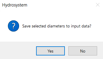
This can happen in two cases: either the change in the input data was not so significant that it led to the selection of other diameter values, or during one of the previous runs of the diameters calculation, you accidentally saved the selected diameters to the input data by clicking "Yes" in the window with the corresponding request:

If the diameters are specified in the input data for branches, then at calculation they are assumed to be known and will not be recalculated (for more information about it, see here), even if you change other input data. Therefore, if you need to "re-select" the diameters for the pipeline, they need to be reset in the input data. To do this, the easiest way is to select all the branches of the pipeline in the tree (using the Shift key) and set the diameters equal to zero in the Object Properties window.

The flowrates in the isothermal or heat analysis results differ from those specified in the input data

This may occur in different cases, let's consider each of them:

1. The flow rate at the start/end point of the pipeline has been recalculated, for which the pressure value is also set. It should be remembered here that the pressure and flow rate in the node are interrelated quantities. If one of them is known, then the other is 'predetermined' by the value of the first one. This can be clearly demonstrated by the example below:

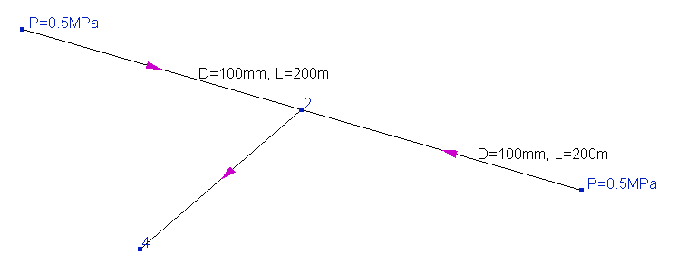
In this pipeline, two streams are mixed at node 2, and the configurations of the branches through which these two streams are fed are exactly the same - they have the same lengths and diameters. Therefore, if the starting pressures in each of these branches are the same (0.5MPa as in this case), then the fluid flowrates for these branches will also be the same. But if, for example, you increase the pressure at one of the starting points, say to 0.6 MPa (and leave 0.5 unchanged at the other), then in this case the flow rate in these branches will no longer be equal. For a branch with an inlet pressure of 0.6 MPa, the flow rate will be larger, since the inlet node of this branch "pushes" the flow harder. That is, the flow rate in the branch directly depends on what pressure is at its beginning (similarly, for the final branch, the flow rate depends on the pressure at its end), and knowing the pressure, you can calculate the flow rate and vice versa, knowing the flow rate, you can determine the pressure. Therefore, if the boundary conditions of the hydraulic calculation are set in such a way that both pressure and flow rate are known for the starting/ending point of the pipeline, such a calculation task is incorrect (for more information about the boundary conditions, see here). This is the same as, for the example above, setting different flowrates values in the branches supplying flows to node 2 - the flowrates in these branches just cannot be different in this piping model at such initial pressures. Their ratio is already predetermined by the pressure values at the initial points of these branches.

The only way to provide the required flow rate in such a branch at a given pressure is to maintain this flow rate using a control valve (for more information about modeling flow regulators, see here) or some other control device. The regulator creates an additional pressure drop, due to which the flow rate is set to the required value at a given pressure. Therefore, if both the pressure and flow at the start/end point of the pipeline need to be as required, the only way to achieve this is to regulate the flow.

If there is no flow regulator in the pipeline, then in order to avoid the above contradiction between the specified flow rates and pressures, the following rule applies in the program - the specified pressure value in the node has a higher priority compared to the flow rate in the adjacent branch. And if both the pressure and the flow rate are set for the starting/ending point of the pipeline at isothermal flow analysis or heat and hydraulic calculation, then the flow rate is discarded and recalculated according to the set pressure value.

Therefore, when setting the boundary conditions of hydraulic calculation, it is most convenient to follow the following rule - for each starting and ending point of the pipeline, either a pressure or flow value must be set. This guarantees the correctness of the formulation of the calculation task being solved.

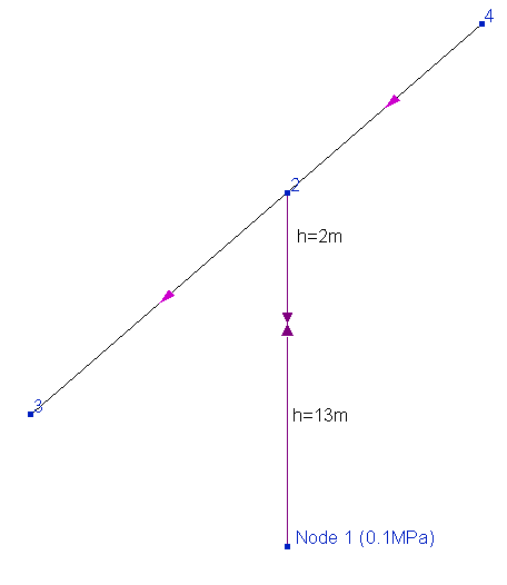
2. The flow rate in the intermediate branch of the pipeline, which is part of the closed loop, has been recalculated. This phenomenon can be clearly demonstrated by the example below:

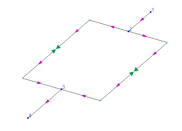
In this pipeline, the flow is supplied from node 1 to node 4, part of the flow goes along the "left" branch of the looped circle, part along the "right" one. And here it is important to understand that the distribution of flows between these branches is predetermined by the configurations of these branches (their diameters, the sizes of their pipes, bends and other components). If the sizes, diameters, etc. of these branches are the same, then the flow will be divided between them equally. If, for example, the "left" branch has a larger diameter or a shorter length (with all other parameters being equal), then the flow capacity of this branch will be greater than in the "right" branch, etc. So, in the calculation for such branches, the flow rates values can not be set in principle - whatever we set them, they will be determined not by our wishes, but by the geometry/characteristics of the branches and their elements.

Therefore, if the required flow value needs to be provided in any branches inside a closed loop, the only way to achieve this is to adjust it using a flow control valve (for more information about modeling flow regulators, see here) or another control device.

3. The flow rate in the intermediate branch of the pipeline, which is not part of the closed loop, has been recalculated. This is either a direct consequence of the recalculation of the flow rate in one of the initial/final branches of the pipeline (see paragraph 1 above), or a simple error in the input data (see paragraph 4 below).

4. A trivial error/typo in the input data. For example, if the flowrates for the branches are set as shown in the figure below, then the flow in the intermediate branch is recalculated, since it is not agreed with the specified flowrates in the initial branches (unless the outflow of 50 m3/h is set for node 2):

The flowrates in the diameters calculation results differ from those specified in the input data

Here, first of all, it is important to remember that during the diameters calculation, in fact, two separate calculations are performed sequentially: the first is the diameters selection itself, and the second is a verification hydraulic calculation of a pipeline with selected diameters (in order to show how a pipeline with selected diameters will operate). Since the hydraulic resistances, and therefore the flow distribution in the pipeline branches, directly depend on the values of the diameters of the branches, it may turn out (and often turns out) that the pipeline with the selected diameters will operate in a slightly different mode from the set one. Either the flow rates will deviate slightly from the set ones (if the consumer pressures are fixed), or the consumer pressures will be slightly higher than the required ones (if the fluid flowrates are fixed). To manage what is considered constant (and what is recalculated) at the verification calculation after selecting diameters, a special option "Flow rate recalculation" is used in the pipeline calculation data.

If this option is enabled, the flowrates in the branches will be recalculated (hence the name of this option), since in this case it is assumed that the pressures set in the input data at the boundaries of the system are fixed and the flowrates are not regulated. That is, in this case, the calculation results will show the real distribution of flows in the pipeline with the selected diameters, provided that there is no flow control.

If the "Flow rate recalculation" option is disabled, then the fluid flow rates specified in the input data are considered fixed and the outlet pressures in the system are recalculated. However, even in this case, flowrates in some branches can still be recalculated. This is due to the discreteness of the selected diameters values at the diameters calculation. The fact is that the diameters are selected from the following list of standard values (if necessary, this list of diameters can be edited in the program settings):

10, 15, 20, 25, 32, 40, 50, 65, 80, 100, 125, 150, 200, 250, 300, 350, 400, 500, 600, 700, 800, 1000, 1100, 1200, 1300, 1400, 1500, 1600, 1700, 1800, 1900, 2000, 2100, 2200, 2300, 2400, 2500, 2700, 2800, 2900, 3000, 3100, 3300, 3400, 3500, 3700, 3900, 4000 mm

That is, the diameter value cannot be "whatever" - it can only be equal to the values from the list above. Therefore, it is often not possible to choose exactly the diameter at which the flow rate in the branch will be exactly as needed. This can be clearly demonstrated by the example below:

In this pipeline, two streams from nodes 1 and 2 mix at node 3 and go to node 4. And it is necessary to select the required diameters of the branches of this pipeline, firstly, so that with such flow rates, the pressure would fall to the end point not lower than the required 0.4 MPa, secondly, so that the flowrates from the sources are distributed exactly in the ratio required (100 and 80 m3/h).

For clarity, let's assume that for this purpose the diameters of the source branches must be at least 100 mm (otherwise the pressure loss will be too large and the flow will not reach the end point with the required pressure), and here the following problem occurs. If we take the same diameters of 100 mm for these two branches, then the flowrates in these branches will be the same - the piping model is absolutely symmetrical, the configurations of these two branches (pipe lengths, types of bends, etc.) are the same, the initial pressures are also the same, therefore the flow rates in them will be equal. If, for example, we take the next larger diameter of 125mm for the branch coming from node 2 (and leave 100mm for the branch coming from node 1), then in this case the flow in this branch will already be greater than in the neighboring one (since it is "easier" for the flow to go through a pipe with a larger diameter). But how much larger it will be depends solely on what diameters this and the neighboring branch will have (flows can be distributed in the ratio 110 to 70, 120 to 60, etc.). And it is often simply impossible to choose such diameters so that the flowrates ratio is exactly 100 to 80, as required.

Of course, it is possible to calculate the exact values of the diameters of these two branches, at which the flowrates on them will be exactly as required. Suppose that we performed such a calculation and got, for example, for the "left" branch (coming from node 2) a diameter of 113.85 mm, and for the "right" branch a diameter of 97.63 mm. But there is no great sense in such a calculation in the first place, since there are no pipes with exactly such diameters in mass production. And anyway, in practice the diameters will have to be 125 for the left and 100 for the right branch (as the closest to the required ones). And with these diameters, the fluid flowrates will be slightly different.

These values (113.85 and 97.63mm) are given here simply as an example - any other values can be used in any other pipeline instead. The point here is that in all cases these will be "non-circular" values (unless you are "lucky" enough), while in piping schedules there are only pipes with "round" values. And it is this "rounding" that is the reason that the flow parameters in a real pipeline will turn out to be different from the required ones.

Therefore, when designing a pipeline, it is only possible to select such diameter values at which the flow rates in the pipeline branches will be as close as possible to the required ones, but not exactly equal to them. The only way to achieve the required flow rate values is then (after the diameters are selected) to adjust them using control valves (for more information about modeling flow control valves, see here) or other control devices.

In the example above, the flow distribution between two source branches is considered, but exactly the same picture will take place for intermediate branches of the pipeline. For example, if there are closed loop in the pipeline, the distribution of flows along branches in such loops also depends on their diameters. Therefore, in this case, it is only possible to choose such diameters at which the flow rates in the branches of the closed loop will be as close as possible to the required values, but it will not be possible to keep them exactly equal to the required ones without flow regulators.

The pressure in the diameters calculation results differ from those specified in the input data

Here, first of all, it is important to remember that during the diameters calculation, in fact, two separate calculations are performed sequentially: the first is the diameters selection itself, and the second is a verification hydraulic calculation of a pipeline with selected diameters (in order to show how a pipeline with selected diameters will operate). Since the hydraulic resistances and flow distribution in the pipeline branches directly depend on the values of the diameters of the branches, it may turn out (and often turns out) that the pipeline with the selected diameters will operate in a slightly different mode from the set one. Either the flow rates will deviate slightly from the set ones (if the consumer pressures are fixed), or the consumer pressures will be slightly higher than the required ones (if the fluid flowrates are fixed). To manage what is considered constant (and what is recalculated) at the verification calculation after selecting diameters, a special option "Flow rate recalculation" is used in the pipeline calculation data.

If the "Flow rate recalculation" option is disabled, then the fluid flow rates specified in the input data are considered fixed and the outlet pressures in the system are recalculated. And indeed, quite often the values of the outlet pressures in this recalculation turn out to be slightly higher than the set ones. This is due to the fact that at the diameters calculation the diameters the diameter of the pipeline is a discrete value. It is selected from the following list of standard values (if necessary, this list of diameters can be edited in the program settings):

That is, the diameter value cannot be "whatever" - it can only be equal to the values from the list above. And in the process of selecting diameters (if you very simplistically imagine its calculation algorithm), the program simply "iterates" the values from the list mentioned above in ascending order until the first (smallest) value is found, at which the pressure loss (the difference between the pressures at the starting and ending points) will fit into the values specified in the input data. And since the nearest larger diameter value is selected, this leads to the fact that with this value the pressure loss will be slightly less than required, which is why the outlet pressure in the pipeline appears to be slightly higher than the set one. This can be clearly demonstrated by the example below:

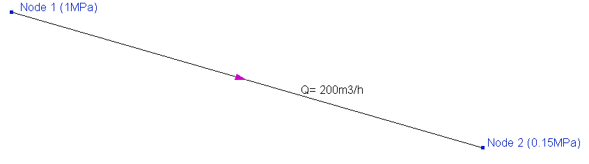
In this example, it is necessary to determine the diameter of the pipeline, at which, when pumping 200 m3/h, the fluid pressure will drop along the pipeline from the initial value of 1MPa to 0.15 MPa. Pressure losses in the pipeline directly depend on the diameter of the pipe and the flow rate (velocity) of the fluid, therefore, it is possible to uniquely determine the diameter value at which the losses in the pipeline will be exactly equal to the required ones. Let's assume that we performed such a calculation and got a diameter value, for example, 174.31mm. Since there are no pipes of such diameters in production (at least in serial), in practice we will have to take either the nearest smaller diameter of 150 or the nearest larger 200mm for this pipe. With a diameter of 150mm, the pressure loss in the pipe will be greater than required (since this diameter is less than required), and with a diameter of 200mm - less than required. Therefore, a diameter of 200 mm is accepted, with which, as a result of reducing hydraulic losses, the pressure at the end point will be slightly higher than the required 0.15MPa.

Thus, due to this "discreteness" of the diameter values, the pressure at the end points of the pipeline (with the "Flow rate recalculation" option disabled), as a rule, turn out to be higher than the set ones. Therefore, in this case it is very important to take into account what is actually located at the end point(s) of the calculated pipeline and what is constant at this point. If the flow rate is constant (for example, it is maintained by a flow regulator), then this difference between the pressure value obtained and the pressure value set in the input data at the outlet point should be interpreted as a pressure drop that the regulator will need to create in order to maintain this flow rate. If the pressure is constant, then you should enable the option "Flow rate recalculation" - in this case, the outlet pressure will be considered constant, and the flow rates will be recalculated.

There is another case that deserves special mention - this is the diameters calculation with a specified fluid velocity limit. It differs from the "usual" diameters calculation in that in this case, after selecting the diameters, the fluid velocity in each branch of the pipeline are checked, and if they exceed the specified limit value somewhere, the diameters in these branches are increased until the velocity will be within the specified limit. In this situation, especially if the diameters had to be greatly increased in order to comply with the fluid velocity limit, the pressure losses may become noticeably lower than required, as a result of which the outlet pressures will be noticeably higher than the set ones. Therefore, it is important to remember that in cases where it is necessary to maintain fluid velocity below some maximum permissible value, it is impossible to do without regulating the flow rate (otherwise, following an increase in diameters, flow rates will also increase, due to which velocities will increase too and it will not be possible to comply with the restriction).

The velocity at the diameters calculation exceed the specified limit

This problem may occur in the following cases:

1. Diameters are set in some branches of the pipeline (possibly by mistake). If the diameter is specified in the input data, then at the diameters calculation it is considered as a known value and will not be "re-selected" (this is used, for example, in cases when the diameters of part of the pipeline branches are known and it is necessary to select diameters only for the rest of the branches). Therefore, it may not be possible to comply with the velocity limit on this branch. In this case, if the diameter was set by mistake, reset it in the input data. If indeed this branch has such a diameter, then it will not be possible to comply with the velocity limit at this flow rate in the branch.

2. The "Flow rate recalculation" option is turned on in the pipeline calculation data. If this option is enabled, it is assumed that the pressures set in the input data at the piping system boundaries are fixed and the flow rates in the pipeline are not regulated (for more information, see here). Therefore, the flow rates in the branches will be recalculated (hence the name of this option). And since the flow rates are not regulated, it is not possible to comply with the velocity limit, since the fluid velocity directly depends on its flow rate. Increasing the diameter of the pipe in this case will not help, because if the fluid flow rate in this pipe is not regulated, then with increasing diameter the flow rate will also increase, and therefore the velocity will increase. Therefore, in order to comply with the velocity limit, the "Flow rate recalculation" option must be disabled (and the flow rates in the pipeline must be regulated).

3. The fluid velocity exceed the specified limit slightly. A slight excess of the maximum permissible velocity is allowed in the calculation (since this is not critical for the operation of the pipeline), if this allows you to choose a noticeably more economical pipeline configuration.

Difference between pressures in terminal nodes is less than the sum of fixed path (...)

If such a message is displayed at the diameters calculation, it means that the pipeline is modeled and the pressure values in it are set in such a way that it is impossible to provide the specified pressure difference at any values of pipe diameters. This can be clearly demonstrated by the example below:

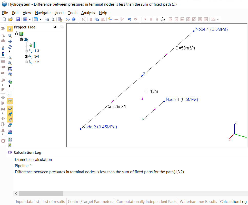
In this pipeline, the pumped fluid is water (with a density of about 1000 kg/m3), which is supplied from node 1 to nodes 2 and 4. And it is required to select what diameters this pipeline branches should have, so that at an initial pressure of 0.5 MPa at node 1, the fluid (moving with a required flow rate) would reach node 2 with a pressure of at least 0.45 MPa, and node 4 with a pressure of at least 0.3 MPa. As you can see, this calculation task has no solution in the first place, since when the flow goes upwards by 12 meters (in the pipe before node 3), at least 12 m*1000 kg/m3 * 9.81m/s2 = 117720Pa will already be lost for hydrostatic losses. Thus, the pressure in node 3 can be a maximum of 0.5-0.11772=0.38228MPa (and most likely it will be even less, since there will also be friction losses and losses on other piping components between nodes 1 and 3). Therefore, it is not possible to deliver the fluid to node 2 with a pressure of 0.45MPa (since the pressure cannot increase along the road from node 3 to node 2).

In order to immediately "cut off" such unsolvable tasks, before the diameters calculation, the program automatically checks the so-called "fixed parts" of pressure losses (hydrostatic losses due to elevation difference, manually set pressure drops, etc.), which will be in the pipeline at any diameter. And if their sum along any of the fluid movement paths turns out to be greater than the difference between the initial and final pressure along this path, the corresponding message is displayed at the calculation and the calculation is interrupted, since there will be no solution to such a task. Therefore, when this message occurs, you should first check:

the correctness of the pipeline geometry - it is possible that the elevation difference for some element is specified incorrectly;
the correctness of the pressure values - it is possible that an incorrect pressure value is set somewhere or the pressure is set in the wrong node in which it is necessary;
the correctness of setting the directions of the pipeline branches - perhaps in some of the branches the flow should go in the opposite direction. For example, if the flow in the pipeline above does not move from node 3 to node 2, but vice versa - from node 2 to node 3, then the calculation task will have a solution.

If all the input data is correct, but this message is still shown, it means that at these pressures in the piping system it is impossible to provide the specified pipeline operating mode.

The results of the isothermal flow calculation performed after the selection of diameters differ from the results of the diameters calculation

As mentioned above, two separate calculations are performed sequentially during the diameters calculation of the pipeline: the first is the selection of diameters, and the second is a verification hydraulic analysis of the pipeline with selected diameters (in order to show how the pipeline with selected diameters will operate). And by default, this verification calculation is performed in order to determine what pressure losses will be in the pipeline with these selected diameters and at the specified flow rates. That is, consumers' flow rates are considered fixed and outlet pressures are recalculated.

If at the diameters calculation the selected diameters are stored in the input data and then an isothermal flow calculation is performed for this pipeline, then this calculation will be performed with other boundary conditions. As already mentioned here, the pressure value in the isothermal flow calculation has a higher priority than the flow rate, therefore, in the isothermal flow calculation, the pressures at the initial and end points (which were set for the diameters calculation) will be considered fixed and the flow rates will be recalculated. Thus, these two calculations have two different goals (in one case, pressure losses are determined at known flow rates, in the other, flow rates are calculated at a known pressure difference), therefore they have different results. In order for the results of the isothermal flow calculation to coincide with the calculation of diameters, it is necessary to reset the final pressures in the input data (or perform the diameters calculation with the "Flow rate recalculation" option enabled).

Non-zero inflow/outflow was calculated at the node

This message can be shown in various cases, let's consider each of them:

1. Flow rates in branches connecting at any node are set in such a way that the sum of inflows and outflows at this node is not zero. This can be clearly demonstrated by the example below:

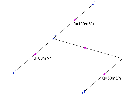
As can be seen, the sum of flow rates entering node 2 (100 m3/h) does not equal the sum of flow rates outgoing from it (50+60=110 m3/h), as a result of which an inflow of 10 m3/h is appeared in the node. Note that, generally speaking, such a formulation of the hydraulic calculation task is quite acceptable. For example, in this way it can be modeled that part of the fluid goes in or goes out of the pipeline at this node (for example, above 10 m3/h is supplied to node 2 "from outside" the pipeline) along some separate branch, the calculation of which is not of interest to the designer. In this case, it is allowed to not model this branch, but simply specify the inflow/outflow at this node (for more information, see here). However, if you did not plan to model such fluid inflow/outflow, then you should check the correctness of the flow rates values in the branches - there may be an error somewhere. Please remember that at the isothermal flow calculation and heat and hydraulic analysis of the pipeline, it is not required for the flow rates to be specified for the intermediate branches of the pipeline (so there's no need to enter them in the input data, especially if you are not sure of their values). Depending on the calculation task (for more information about this, see here), it is enough to set the flow rates either only in all inlet branches or only in all outlet branches.

2. The pressure is set in the intermediate node of the pipeline. In hydraulic calculation in a Hydrosystem, the pressure value has a higher priority than the flow rate (for more information, see here), therefore, if pressure is set in some intermediate node, then the flow rates in the branches adjacent to it can be recalculated according to this pressure value and their balance in this node may not converge. This can be clearly demonstrated by the example below:

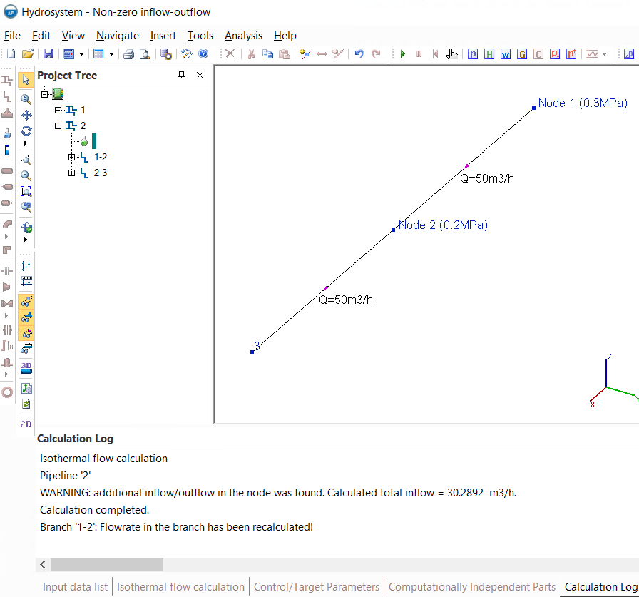
In this pipeline, the fluid is supplied from node 1 (with a pressure of 0.3MPa) to node 3 with a flow rate of 50 m3/h. And at the same time, for some unknown reason, the pressure is also set in the intermediate node 2 (0.2 MPa). In this case, the flow rate in the first branch (connecting nodes 1 and 2) will be recalculated by the pressure difference in these nodes (0.3 minus 0.2MPa), and the calculation of the second branch (connecting nodes 2 and 3) will be performed with the flow rate set in the input data of 50 m3/h. As a result, it turns out that in the first branch the flow rate is about 80.2892 m3/h (in fact, this is the flow capacity of this branch at a given pressure difference), in the second 50 m3/h - that is, in node 2 the outflow of fluid is 30.2892 m3/h. Thus, by setting the pressure in the intermediate node, you can get a completely incorrect piping calculation model. Therefore, please note that in hydraulic calculations, depending on the formulation of the calculation task to be solved, it is necessary to set the pressure either only at the inlet points, or only at the outlet points, or both at the inlet and outlet points of the pipeline (for more information about this, see here), but not in intermediate ones.

At this stage of the reasoning, a logical question may arise: if indeed setting the pressure in the intermediate node of the pipeline is so "harmful" and can distort the piping calculation model so much, then why don't the Hydrosystem developers block the specifying pressure for intermediate nodes or ignore it at calculation or something like this? Well, the answer is very simple - in some cases, setting the pressure in the intermediate node can be of practical use. This can be clearly demonstrated by the example below:

In this pipeline, two streams from nodes 1 and 3 are fed into the equipment indicated in the diagram by node 2. That is, physically, this equipment has two inlet pipes into which the fluid enters, and the pressure in this device is constant and known. And it turns out that although formally node 2 is an intermediate node of the pipeline (since more than one branch is connected to it), in fact it is the final consumer node. Therefore, in such pipelines, it may be necessary to set the pressure in the "intermediate" node. In this case, the calculated amount of inflow/outflow in this node will correspond to the amount of fluid entering the equipment.

The inflow/outflow cannot be specified in nodes with tees

Why inflows/outflows may occur in pipeline nodes and how to deal with them is described in detail here. But if for a node that does not have a tee, this message is just a warning that does not interfere with the calculation, then if there is a tee in the node with an inflow/outflow, the calculation is interrupted with a corresponding error. This is due to the fact that the hydraulic resistance of the tee largely depends on the ratio of flows going in and out of each of tee leg. And if the sum of the inflows/outflows in the tee is not zero, it is impossible to calculate it.

Therefore, if this error occurs, it is necessary to eliminate the inflow/outflow that occurs in the node with the tee, then repeat the calculation. If, for some reason, the elimination of this inflow/outflow is not possible, you can remove the tee from this node - in this case, the calculation will be performed with this inflow/outflow.

What's the difference between inflow/outflow in a node and the flow rate in a branch

If the terminal node of the pipeline (that is, the initial or final node) is concerned, then the inflow/outflow at this node is essentially the same as the flow rate in a branch that starts/ends in this node. For example, if you need to calculate the pipeline in the figure below with the specified flow rates, then you can either set outflows at nodes 3 and 4, respectively, 100 and 120 m3/h, or set a flow rate of 100 m3/h in the branch connecting nodes 2 and 3, and a flow rate of 120 m3/h in the branch connecting nodes 2 and 4:

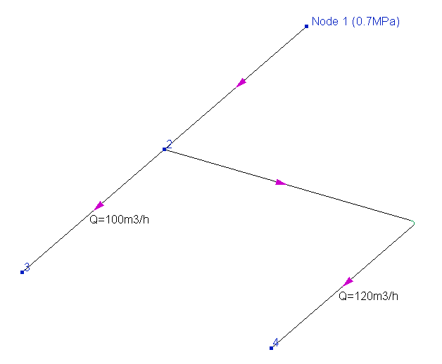
Both will be right - it's just a matter of convenience. The main thing here is not to get messed up with the signs of inflow and outflow ("+" - outflow, the flow goes out from the pipeline; "-" - inflow, the flow is supplied to the pipeline "from the outside") and not forget to set the temperatures of the inflow in the corresponding field. In addition, it is not allowed to specify inflow/outflows in nodes when calculating multiphase flows - in this case, you should specify the flow rates in branches.

A negative flowrate in the calculation results

The flow rate with a minus sign in the branch, as already mentioned here, should be interpreted as the flow going in the direction opposite to the direction of the branch itself. A negative value of the flow rate in the calculation results may indicate both, some peculiarities of the pipeline modeling and possible problems in the operation of this pipeline. For clarity, let's consider each of these two cases separately.

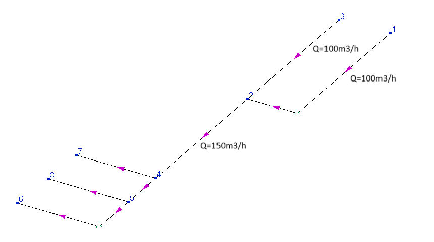
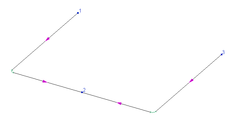
On the figure below a pipeline in which the flow is supplied from node 1 to consumers in nodes 3, 6, 7 and 8 is shown:

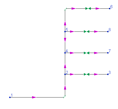
As can be seen in the diagram (by the arrows showing the directions of the branches), an 'error' was made when modeling this pipeline, namely, the branch connecting nodes 4 and 5 is directed from node 5 to node 4, although the flow, of course, will go in the opposite direction - from node 4 to node 5. When calculating such a pipeline, in this branch you will get a flow rate with a minus sign, but it is important to understand that in fact, as such, this is not an "error". When performing isothermal flow calculations and heat and hydraulic calculations of pipelines, the directions of the intermediate branches are not of fundamental importance for the calculation, therefore, even if some branches are modeled "backwards", this will not affect the correctness of the calculation. If you want to "get rid" of minus signs of the flow rates in such branches, use the "Reverse direction" command in the context menu, which is called by right-clicking on a branch in the project tree (or the corresponding Edit menu item). When changing the direction of the branch, it is "redrawn" in the opposite direction (its end node becomes the starting one, and the starting one becomes the end one), and after that the calculation of the pipeline is repeated, the results will be the same, but this time the direction of the branch and the direction of flow in it will coincide and the flow rate will be positive. However, it is not necessary to do this, because as mentioned above, this will not affect the correctness of the calculation in any way. So it's just a matter of convenience (so that the "minus" sings of the flow rates do not cause unnecessary questions).

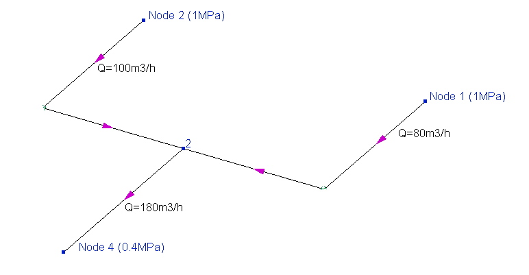
And the picture below shows a different situation. In this pipeline, the flow from the source node 1 is supplied to two consumers (nodes 3 and 4), and known pressures at the initial and final nodes of the pipeline are set as boundary conditions for calculation:

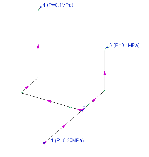
And if, when calculating such a pipeline, the flow rate, for example, in the branch connecting nodes 2 and 4, turns out to be negative in the calculation results, then this means that the flow "cannot rise up" from node 2 to node 4 (due to a large column of liquid on the vertical section of the pipe in this branch). Unlike the previous example, in this case, a negative flow rate indicates errors in the design of the pipeline system, due to which it is in principle unable to operate in the required mode.

Thus, each case in which negative flow rate values are obtained in the calculation results on any branches should be considered individually and analyzed whether this is a simple flaw in the modeling of the pipeline or whether this indicates problems in the operation of this pipeline.

The pressure is negative or too low

If such a message is displayed at the calculation, it means that if the fluid were pumped with flow parameters (pressures, flow rates) set as boundary conditions and with the pipe fully filled, then by some point in the pipeline the pressure would fall below absolute vacuum. Since this is physically impossible, this message should be interpreted as saying that the fully filled pipe flow with the specified parameters is impossible.

It is important to take into account here that since in calculations in the Hydrosystem it is considered that the pipe is fully filled with the pumped fluid, this message should be interpreted as the impossibility of pipe flow (where the whole cross-section of the pipe is filled with fluid) in the pipeline under these conditions. However, a flow with free surface (where not the whole cross-section of the pipe is filled with fluid) with these parameters may either exist or not, depending on the conditions. To distinguish these situations from each other, let's look at each of them with an example.

Below is an example of calculating a pipeline in which the fluid is supplied from the starting point 1 with a pressure of 0.3MPa (abs.) to the end point 3 with an atmospheric pressure of 0.1MPa abs. (the main input data and results of this calculation can be seen on the "Isothermal flow calculation" tab below):

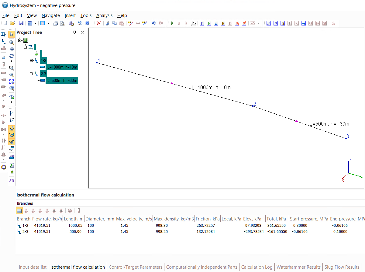
First, the flow goes in a 1000 m long pipe with an upward slope, rising to point 2 by 10 meters, then from point 2 to point 3 with a downward slope of 30 meters along a 500 m long pipe. The inner diameter of the pipe is 100mm, the product is "Water/steam by IAPWS-IF97" with a temperature of 20C (in case you want to model this pipeline system yourself).

As can be seen from the results of the isothermal flow calculation of this pipeline, the pressure at point 2 is -0.06166 MPa (abs.), that is, below the absolute vacuum. As mentioned above, this should definitely be interpreted as the fact that the pipe flow (with the whole cross-section of the pipe filled with the fluid) in the pipeline with these parameters is not feasible. Now let's find out if there can be (and with what parameters) a flow with free surface in such a pipeline. It is quite simple to check this - you need to set the atmospheric pressure (0.1MPa abs.) at the point with the lowest pressure in the pipeline (that is, the highest located point in it) and repeat the calculation. The logic here is that if the calculation results show a positive flow value between points 1 and 2, this means that the fluid pressure is sufficient to fill the pipeline and rise to the highest point in the pipeline and move with this flow rate. Setting pressure 0.1MPa (abs.) in the 2nd node of the pipeline (judging by the diagram, it is the highest point in the pipeline) we will get the following results:

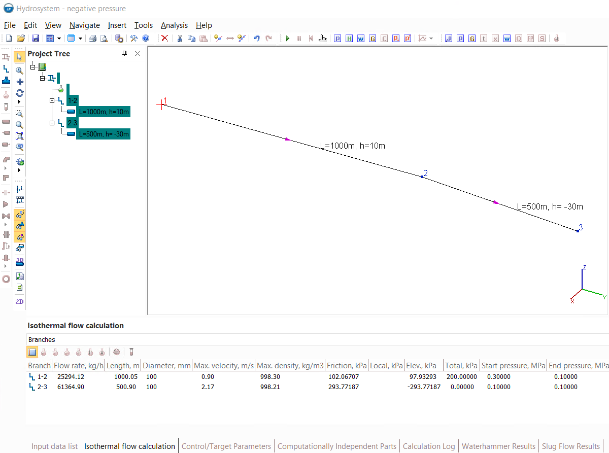
As you can see, the flow rate in the first branch is about 25,000 kg/h, that is, if in an empty pipeline (with an atmospheric pressure of 0.1MPa abs.) a fluid with a pressure of 0.3MPa (abs.) at the starting point is supplied, then it will move with a full filling of the pipe section with a flow rate of about 25,000 kg/h to point 2. Further, the fluid flow rate from point 2 to point 3 in the calculation results is 61364.9 kg/ h, that is, more than the flow rate before point 2. To correctly understand this value, it should be remembered that, as mentioned above, the Hydrosystem considers any flow as a fully filled pipe flow. That is, this value should be interpreted in such a way that at atmospheric pressure at points 2 and 3 (0.1MPa abs.) the pipe flow with full filling of the pipe between these two points in this pipeline would be established with a flow rate of 61364.9kg/h. And since the flow rate of the fluid that came to point 2 from the beginning of the pipeline is less than this value (it is only 25294.12 kg/h), then there will be no complete filling of the pipe, since the fluid cannot come 'from out of nowhere' in the pipeline (how much fluid entered at the beginning of the pipeline, that much will come out from it at the end). Thus, a fully filled pipe flow will be established only on the first part of the pipeline from node 1 to node 2, and then from node 2 to node 3 there will be a free surface flow with a flow rate of 25294.12 kg/h.

Now let's consider the same pipeline system, but in which the inlet pressure, for example, is 0.15MPa (instead of 0.3MPa). After calculating the system with such parameters, we will get the following results:

This time, the fluid flow rate between points 1 and 2 will be negative (-17122.52kg/h). Again, in order to correctly understand this value, it should be remembered that the Hydrosystem considers this flow as a fully filled pipe flow. That is, this value should be interpreted in such a way that at a pressure of 0.15MPa abs. at point 1 and a pressure of 0.1MPa abs. (i.e. atmospheric) at point 2 and when the pipeline is fully filled with the pumped fluid, the flow will not move from point 1 to point 2, but backwards with a flow rate of 17122.52kg/ch. That is, the initial flow pressure is not enough to raise the fluid to point 2 with any flow rate, and the flow in the pipeline with these parameters is impossible (neither fully filled flow nor the free surface flow). Physically, this means that if a fluid with a pressure of 0.15MPa (abs.) is fed into an empty pipeline (with an atmospheric pressure of 0.1MPa) at the starting point, it will fill only part of this pipeline and stop at some height (that is easy to calculate by subtracting from the initial pressure of 0.15MPa (abs.) the atmospheric pressure is 0.1MPa abs. and dividing this difference by the density of the fluid and the acceleration of gravity is 9.81m/s2).

Thus, the message about the negative pressure in the calculation, depending on the situation, may indicate both the fundamental impossibility of the flow and a change in its nature from a flow with full pipe fulfillment to the flow with a free surface. And in the shown above way, you can distinguish one situation from another.

In addition, the approach described above can also be used for "reverse" calculation - that is, if for the above pipeline system you need to calculate what pressure should be at the beginning of the pipeline so that the required flow rate of the fluid can be pumped into this pipeline, then it's necessary to set the atmospheric pressure of 0.1MPa abs in node 2, specify the required flow rate in the first branch of the pipeline and do not set the pressure in node 1 - it will then be determined at the calculation.

Violation of the flow continuity

This message is shown in cases where the pressure in the pipeline is set in such a way that in some of its closed parts there is a pressure below absolute vacuum. Since this is physically impossible, this message should be interpreted as the fact that the pipeline will not be completely filled with the pumped fluid with the specified parameters. This can be clearly demonstrated by the example below:

The fluid in this pipeline is water (with a density of about 1000 kg/m3), an atmospheric pressure of 0.1MPa (abs.) is set in node 1 at the bottom, the valve in the branch connecting nodes 1 and 2 is closed. Obviously, in practice, such a situation is not feasible when the pipeline is completely filled with the pumped fluid, since in this case the fluid pressure in the point at the bottom of the closed valve should be 0.1 MPa - (1000kg/m3*9.81m/s2*13m)/1000000 = -0.02753 MPa abs., that is, below the absolute vacuum. Therefore, this is possible only if the pipeline is not fully filled with fluid (or an empty pipeline), that is, if the continuity of the flow is violated.

If you only need to perform a steady-state flow calculation (isothermal flow calculation, heat and hydraulic analysis or diameters calculation), you can ignore this message. Since the part of the pipeline in which the pipeline is partially filled with the fluid is cut off from the rest of the system and has no effect on it. However, to perform the calculation of a waterhammer, this phenomenon is unacceptable, since in a Hydrosystem, the calculation of a waterhammer can adequately describe only those processes that occur in pipeline systems fully filled with the pumped fluid. Therefore, the calculation of the waterhammer in such a system will not be performed.

Mach number > 1, a chocked flow in the pipeline

One of the limitations of Hydrosystem (for more information about the limitations of the program, see here) is its operability only in the so-called "subsonic" flow region, when the flow Mach numbers do not exceed about 0.7 (that is, the fluid velocity is less than 70% of the speed of sound). If the input data for the calculation are set in such a way that flow velocities above 0.7 of the speed of sound occur at some points in the pipeline, then high accuracy of such calculation is not guaranteed, since the program methods are not designed to calculate such cases (and often the calculation in this case will not converge at all and will be interrupted with an error).

Therefore, if such a message occurs during the calculation, first of all it is necessary to check the correctness of the input data (first of all, the values of diameters, flow rates and pressures). Usually, when designing pipeline systems for various purposes, it is recommended to avoid high fluid velocities, since high velocities are unprofitable, both from the point of view of efficiency (pressure losses at pumping will be very high, which will lead to increased energy costs for compressors, pumps, etc.), and from the point of view of safety (at high speeds, the occurrence of electric charge on the pipeline due to fluid friction), and in terms of noise, etc. Therefore, in a "well-designed" pipeline system, there should be no fluid velocities of the same order as the speed of sound. Exceptions to this rule are pipelines of emergency discharge systems (where the fluid velocities can be very high) and pipelines in which gas-liquid mixtures with comparable volumes of liquid and gas phases are pumped (for example, "transfer" pipelines for supplying petroleum to a distillation column in a vapor-liquid state). In such pipelines, the fluid velocities in practice can be very high, up to sound. For calculations of such types of pipelines, a special "reverse" calculation tool is provided in Hydrosystem, which allows for pipelines with an "Undefined" fluid phase state and consisting of a single branch to perform heat and hydraulic calculation, including near-chocked (with Mach numbers 0.7<M<1) and chocked flow (with Mach number M=1). More details about this calculation are described here.

As for all other types of pipelines, at the moment the possibility of calculating near-chocked and chocked flow is not provided for them.

Please note that in some cases, the message about high Mach numbers in the calculation may be a consequence of another, more "banal" problem - pressure drop along the pipeline to values close to absolute vacuum. The fact is that the speed of sound in a fluid directly depends on the pressure, and the fluid velocity itself depends on it too (especially for gases and gas-liquid mixtures) - the lower the pressure, the lower the density of the fluid and the higher its velocity will be. And this dependence becomes more and more "sharp" as the pressure approaches zero. Thus, if the fluid pressure drops low enough, the consequence may be an increase in the fluid velocity to sonic velocity. Therefore, if this message is displayed at the calculation, it also makes sense to check how much the pressure changes along the pipeline (for example, by "shortening" the pipeline and calculating pressure losses only for its small initial part) and whether it has fallen "to zero".

A phase transition has occurred, the wrong fluid phase state

The Hydrosystem provides a special system for diagnosing the fluid phase state. Therefore, if during the calculation it turns out that the phase state of the fluid changes along the pipeline (for example, the gaseous fluid has cooled down to the condensation temperature or the pressure of the liquid stream has dropped to the boiling pressure, etc.), the program outputs the corresponding message during the calculation. If the "Liquid" or "Gas" phase state is set for the fluid, then the results of such calculation (if it was possible to perform it) should be treated with caution, since when explicitly specifying the fluid phase state (liquid or gas), the calculation is carried out using single-phase flow methods that do not take into account the effects of boiling, condensation and etc. in pipeline. Therefore, in this case, you should choose an "Undefined" fluid phase state, when using which these effects are taken into account in the calculation (for more information about the fluid phase states, see here).

The fluid phase state can only be checked when modeling the pumped fluid using the thermodynamic libraries STARS, GERG-2008, WaterSteamPro (Water/Steam by IAPWS-IF97) and Simulis Thermodynamics. Moreover, for the first two libraries, this check can be disabled if necessary (for example, if you are sure that condensation/boiling of the fluid will occur only to a small extent along the flow, and it can be neglected without significant error in calculation results) by disabling the corresponding option in the fluid parameters.

In addition, the fluid phase state check is also performed for the inlet flow parameters. Therefore, if, for example, one phase state is set for a fluid and at the same time in some branch of the pipeline the pressure and temperature are set in such a way that the fluid is in a different state at these parameters, then the calculation in this case will be interrupted with a corresponding error. In this case, it is necessary to check the correctness of setting the flow pressure and temperature, as well as the composition and phase state of the fluid.

The pipeline contains unconnected parts with insufficient data for calculation..., The system splits into disconnected parts...

Such errors can occur in the following cases:

1. There are two or more parts in the pipeline that are not "physically" connected to each other in any way (that is, they do not have a single common node) and in one of them the pressure is not specified in at least one point. This may occur if mistakes were made when modeling the pipeline. For example, if a user accidentally deleted a branch or branches connecting different parts of the pipeline (as a result of which they became unconnected) or set incorrect numbers of start/end nodes to some branches. In this case it is impossible to calculate that part in which pressure is not specified, so you need to specify the pressure in at least one point in each of these unconnected pipeline parts and then run the calculation.

2. The pipeline has a closed valve that "divides" the pipeline into parts independent of each other, and at least one of these parts the pressure is not specified in at least one point. In this case, it is not possible to perform the calculation for this part. Therefore, it is necessary that the pressure be set at least in one point in each independent part of the pipeline.

3. There are control valves in the pipeline, and somewhere either before or after one of these valves, the pressure in the pipeline is not set at any point. When calculating pipelines with flow regulators, the parts of the pipeline before and after each regulator are calculated independently of each other (for more information about this, see here), therefore, it is necessary that the pressure be set at least in one point in each of these parts.

To understand exactly which independent parts the pipeline model consists of, how they are connected (or not connected), and what data is missing for calculation, use a special service for topological analysis of the pipeline, which is described in more detail here.

Negative pressure drop on the control valve

If such a message is displayed during the calculation, first of all it is necessary to recall the principle of operation of the control valve. A control valve in a Hydrosystem means a flow control device, and its operation can be simplified as follows: it creates an additional pressure drop at the place of its installation, thanks to which the fluid flow rate is set to the required value. In other words, the control valve "squeezes" the pipeline just enough to provide the required flow rate. And the calculation of the control valve comes down to determining exactly how much the flow needs to be "squeezed" (what pressure drop should be at a given point in the pipeline) so that the flow rate turns out to be as required.

Therefore, if during the calculation it turns out that the pressure drop on the control valve is negative, this means that the flow does not need to be "squeezed", but on the contrary - it is necessary to apply an additional pressure to the fluid so that it is pumped at the required flow rate. Thus, this message should be understood as the fact that with the specified flow parameters, the control valve is not able to provide the required flow rate in the pipeline - it is necessary either to use a more powerful pump for pumping, or to change the configuration of the pipeline, otherwise the flow rate in the pipeline will be less than required.

Please note that since the calculated value of this negative pressure drop on the control valve corresponds exactly to the pressure difference that is not enough to pump the fluid with the required flow rate, this opens up one interesting "undeclared" function of the program - the "Control valve" element can be used not only to determine the settings of the flow regulator, but also for calculation of the required pump head for pumping. That is, the pump must be modeled as a control valve and set the required flow rate on it, and the negative pressure drop obtained in the calculation results will represent the required pump head.

What the abbreviations of two-phase flow patterns stand for

After performing the calculation of two-phase and three-phase flows, you can enable the display of flow patterns in the diagram (for more information, see here), so that the elements of the pipeline are painted in different colors, depending on what gas-liquid flow pattern is established on them. And the "legend" with the designation of the color corresponding to each flow pattern looks like this:

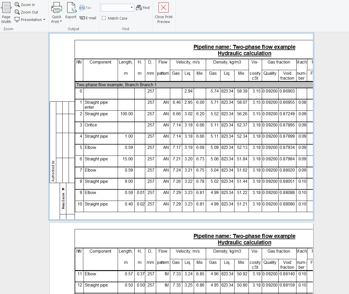
Unfortunately, it is not convenient to fully describe the name of each of the flow patterns opposite its color (the names of the modes are very long and it will not be possible to fit them there). The interpretation of these abbreviations can be viewed as follows - preview a report with detailed results for two-phase or three-phase flow (using the button "Print forms - Print Detailed Results" of the Main toolbar or the corresponding item of "Analysis" menu) and you will find the list of all flow patterns and their abbreviations at the lower left area of the first sheet of this report:

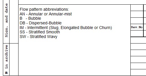
The remaining designations are not flow patterns as such: L - liquid, for elements with only a liquid phase, V - vapor, for elements with only a vapor phase, U - undefined, for elements with an undefined flow pattern (for example, for piping components with phase transition - see here).

The two-phase flow pattern was not determined at some piping component

In some cases, for two-phase flows when showing flow patterns, an "undefined" flow mode may be displayed on the diagram for some piping components:

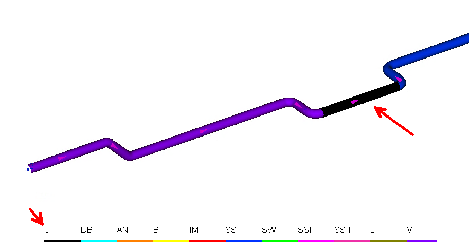
This should be interpreted as the fact that there is a change in the phase state of the fluid (phase transition) at this piping component - the gas or liquid passes into a two-phase region or vice versa. In this case, there will be a single-phase flow for part of this piping component, and a two-phase flow for the other part, so it is impossible to determine an unambiguous flow pattern for this piping component.

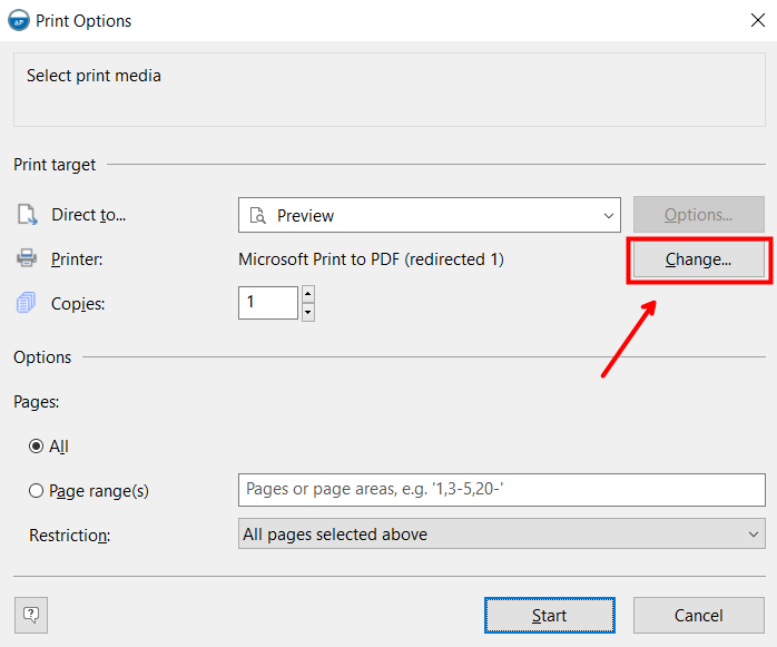
When printing the results, part of the document is ''cut off''

In some cases, when displaying a report in preview or when printing to a file, it may look something like this:

This may occur if a printer that does not support the required print format is used for printing (for example, the document has A3 format, and the printer supports printing only on A4). To get around this problem, simply select any other printer in the print settings (possibly a "virtual" one, like "Microsoft Print to PDF", "OneNote" or similar):

Elevation mismatches found at the calculation

If this message is displayed at the calculation, it means that vertical projections and elevation differences are incorrectly/inaccurately set on some elements of the closed loop of the pipeline. What this means for the calculation and how to find and eliminate these inconsistencies are described in detail here.

At parameters selection the number of goal parameters should be equal to the number of control ones

This message is displayed if a different number of target and control parameters are set for the parameters selection. If your plans did not include performing a calculation with the parameters selection (for more information about this calculation, see here), then you most likely just mistakenly enabled the parameters selection for some pipeline elements. To disable it, you need to do the following:

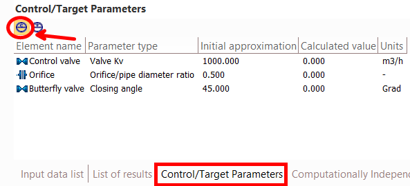
1. Open the Control/Target Parameters window

2. In the upper-left part of this window, click on the first (left) switch button. In this case, a list of pipeline elements for which control parameters are set will be displayed in the window (if this list is empty, go to step 4):

3. Select each of the pipeline elements in this list one by one, open the "Parameters Selection" tab in the Object Properties window for the selected element and disable all enabled checkboxes on it.

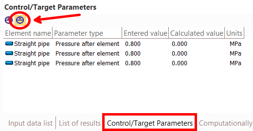
4. In the upper-left part of the control-target parameters window, click on the second (right) switch button. In this case, the window will display a list of pipeline elements for which target parameters are set (if this list is empty, go to step 6):

5. Select each of the pipeline elements in this list one by one, open the "Parameters Selection" tab in the Object Properties window for the selected element and disable all enabled checkboxes on it.

6. Repeat the pipeline calculation.

The viewpoint is too close to the active or reflection node

Such a message may be shown in cases where the location of the viewpoint is selected in such a way that, with the specified waterhammer calculation settings (the calculation step and the data output step - see more about this here), it is impossible to ensure sufficient accuracy in calculating the flow parameters during a waterhammer for this point. This can be clearly shown in the example below:

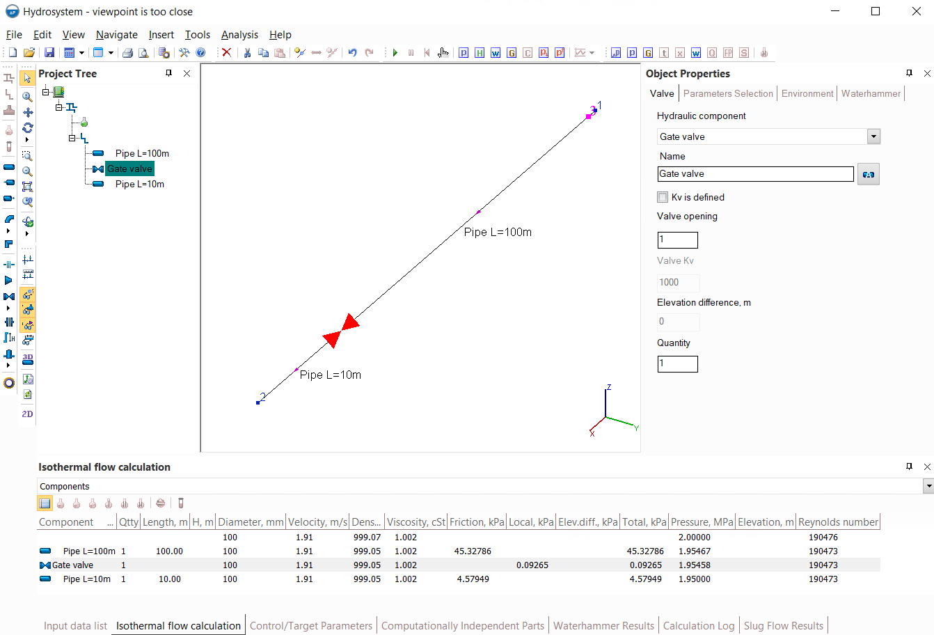
In this pipeline, the fluid (water with a temperature of 20C, modeled as "Water/steam by IAPWS-IF97") is pumped from node 1 to node 2, and a waterhammer calculation is performed for the scenario of instant closure of the valve at the end of this pipeline. The conditions are modeled in such a way that the velocity of the shock wave propagation at waterhammer is 1000 m/s, the data output step is set to 0.1 seconds, the viewpoint is located at a distance of 3 m from the beginning of the pipeline (from the reflection node).

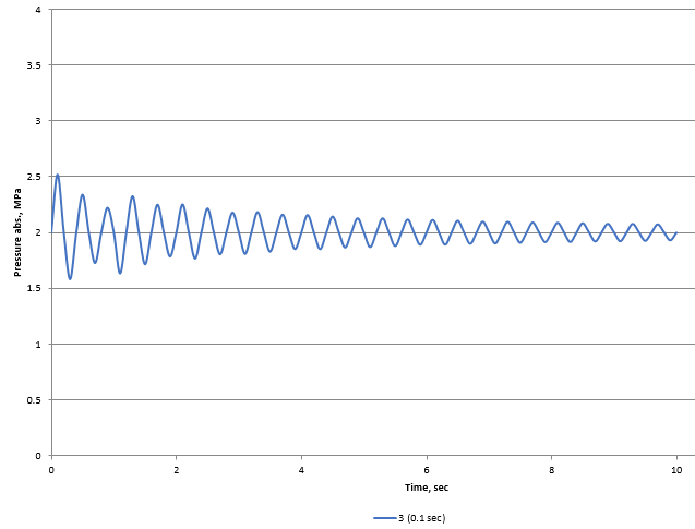
As described in detail here, the waterhammer calculation step is taken equal to the lesser of two values - the ratio of the length of the shortest pipe section in the pipeline to the shock wave velocity (for this example, it will be 10m / 1000m/s = 0.01 sec) and the specified data output step (0.1 sec), i.e. in this case, the calculation step is 0.01sec. Thus, the length step in calculating the flow parameters (pressure, flow rate, etc.) at a waterhammer transient process will be 1000 m/s * 0.01 s = 10m. That is, it turns out that the viewpoint is located at a distance (3m) from the reflection node which is less than the first point in the pipeline for which the flow parameters (10m) will be calculated. In this case, it is impossible to guarantee sufficient accuracy of the calculation for this point. This phenomenon can be clearly demonstrated on pressure charts for this viewpoint - here is this chart with the initial calculation settings (with a calculation step of 0.01 and a data output step of 0.1 seconds):

And here is the chart for the same viewpoint but with higher accuracy of calculation (with a calculation and output step of 0.001 seconds):

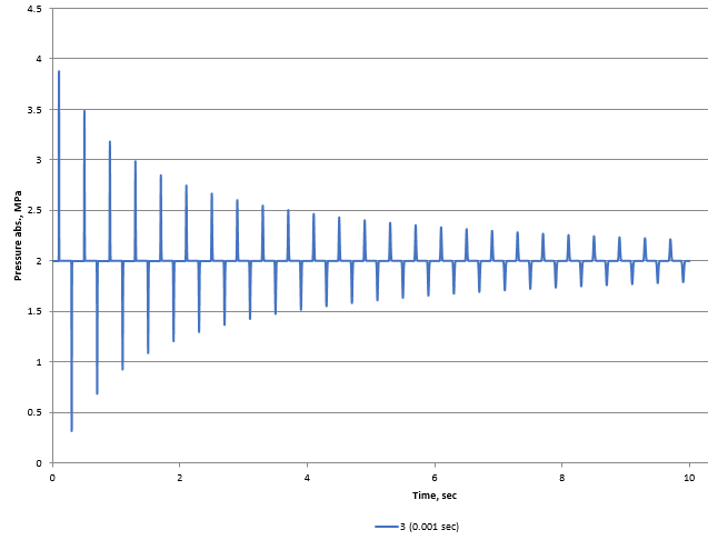
As can be seen, in the first case, the amplitude of pressure oscillations is much smaller than in the second. This is due to the fact that the pressure spikes are very "cut off", since they cannot be accurately registered with the specified calculation settings. In other words, the duration of the pressure increase at this point turns out to be less than the calculation step, that is, the pressure increases so briefly that its peak value is simply "skipped" due to the output step is not small enough to correctly determine it. That is why in such situations, the program warns that the results for a given point may not be accurate.

There are two ways to get around this problem: the first, which logically follows from the reasoning above, is to reduce the data output step (which will lead to a decrease in the calculation step), that is, to perform the calculation with greater accuracy. However, it should be remembered that reducing the step can greatly slow down the progress of the calculation, which may be unacceptable for complex and lengthy pipeline systems. Therefore, in practice, another method is also widely used - it is to place viewpoints at some distance from the nodes of reflection of shock waves and active elements (closing/opening valves and starting/tripping pumps). The fact is that when passing even several tens of meters in a pipe, the force of the shock wave usually practically does not change, since the loss of its energy is incomparably small compared to the energy of a waterhammer. Therefore, the peak values of pressures and other flow parameters at this point will be almost the same as directly next to the reflection node/active element, but at this distance these peaks will be much easier to accurately record. For example, this is how the pressure graph looks for the same calculation above (with a data output step of 0.1 sec), but for a viewpoint located 20 meters from the starting point of the pipeline:

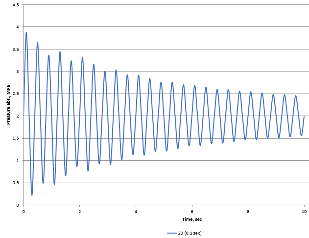
As can be seen, the peaks of pressure oscillations in this case are a little "cut off" too, but their values almost exactly correspond to the peaks obtained in the calculation with a much smaller step of 0.001s. Thus, by placing the viewpoints at a certain distance from the reflection nodes and active elements, it is possible to achieve the required calculation accuracy with much less calculation time.

Note 1: it is important to remember that, as a rule, near the active element (closing/opening valves and starting/tripping pumps) there are short-term oscillations in the flow rate of the liquid (it is almost motionless and only for a very short time it "twitches" a little bit during the passage of the shock wave), and the phases of pressure increase/decrease, on the contrary, are quite long. And near the reflection node with constant pressure (the starting or ending point of the pipeline), on the contrary, pressure oscillations are short-lived, and oscillations of the liquid itself (its flow rate) are prolonged. This should be taken into account when performing the calculation of the waterhammer. Therefore, if, for example, the purpose of your calculation is to determine peak pressure values near a closing valve, then this value will be easy to register even with a large calculation step and even if the viewpoint is very close to this valve (since the increased pressure at the valve will last for quite a long time). Similarly, to determine peak flow rates/velocities, it is safe to place viewpoints close to the inlet/outlet nodes of the pipeline, since the movement of liquid at this point will be quite prolonged at a waterhammer.

Note 2: all the above-mentioned effects are usually noticeable only with a rather abrupt nature of the events causing the waterhammer (for example, with instant or very fast opening/closing of the valve). Therefore, if a waterhammer caused by a smooth event is calculated, this problem may not exist at all, since in this case the phases of pressure increase/decrease and flow oscillations will be quite long at all points of the pipeline.

The calculation of the waterhammer takes a very long time

As described in detail here, the waterhammer calculation speed strongly depends on the calculation step, which is selected as the lesser of two values - the ratio of the length of the shortest pipe section in the pipeline to the velocity of the shock wave propagation and the data output step set in the calculation settings. Therefore, the first thing that should be done to speed up the calculation is to select the optimal data output step (see here), with the required calculation accuracy will be achieved at the highest possible calculation speed.

However, even if you set a fairly large data output step, the calculation of the waterhammer can still take a long time if there are sections of pipes with a small length in the pipeline. This is due to the fact that with such short pipes in the model, the calculation step has to be taken less so that the shock wave is "registered" in each of these sections at least once. This leads to a noticeable slowdown in the waterhammer calculation (in such cases even a corresponding warning is displayed at running the waterhammer analysis that the calculation of the waterhammer for pipelines with such a short pipes sections may take a long time).

Therefore, in order to increase the speed of waterhammer calculation, it is recommended to:

1) avoid modeling separate short pipe sections in the pipeline (separated from other pipes by other elements - bends, valves, etc.). If there are short sections in the piping model, it is better to model them not as separate elements, but to add their lengths to the lengths of adjacent longer pipe sections or not to take them into account in the calculation at all (if their resistances are incomparably small compared to other elements of the pipeline);

2) avoid specifying bends, elbows and reducers in the pipeline that are not surrounded on both sides by pipe sections. If a bend/elbow or reducer is surrounded by straight pipes, in this case it can be considered in the calculation as a "point" dimensionless resistance, and then its presence will not lead to a slowdown in the calculation of waterhammer. If the bend/elbow/reducer is not surrounded by pipes on both sides (for example, if there are the two elbows in a row, or an elbow immediately after the reducer, or the bend/elbow/reducer is specified as the first/last element in the branch), it must be considered in the calculation of waterhammer as an element with length, and therefore it will slow down the calculation of waterhammer, since the length of the bend/elbow/reducer is usually small.

In the absence of such elements in the piping model, the calculation accuracy will not significantly suffer, but the waterhammer calculation speed will increase significantly, since the calculation step will become larger.

Elevations and angles haven't been recalculated on graphics because the current pipeline is not displayed, or…

As described in detail here, the Hydrosystem provides the ability, when starting the pipeline calculation, to automatically recalculate the elevation differences on the pipeline elements, the angles of bends and elbows and other geometric characteristics of the elements according to their graphical representation in the graphic window. However, this recalculation cannot be performed in cases when some "unsuitable" pipeline representation modes are selected in the graphics parameters (for example, if "Show all components" option is disabled or the piping model is displayed in the "Simple scheme" mode or there are closed loops in the pipeline and the "Scaled graphic view" pipeline representation option is disabled, etc.). In this case, a corresponding message is displayed during the calculation.

Therefore, if you are sure that you have specified all the geometric characteristics of the piping components correctly and have not missed anything, then this message can be ignored. If you doubt whether the elevation differences are correctly set for all elements, whether the angles of bends are correctly set, etc., then:

enable the "Scaled graphic view" and "Show all components" options in the graphics settings, if they are disabled;
make sure that the "Precise graphic representation of scaled view" option is enabled in the program settings;
select the pipeline to be calculated or any of its elements so that its diagram is displayed in the graphics window;
repeat the pipeline calculation.

In this case, the recalculation by graphics will be performed before the pipeline calculation.

There is an apparatus with known pressure drop in the branch with flow not specified

Since the hydraulic resistance of any element of the pipeline or equipment depends on the flow rate of the fluid flowing through it, it is strongly not recommended to use the element "Component with known change of pressure and/or temperature" in pipeline branches for which the flow rate is unknown. The fact is that the change of pressure of this element is assumed to be constant in the calculation, that is, independent of the flow rate, which is completely untrue. Such an assumption (about the constancy of this change of pressure) can lead to a serious calculation error (more about this is described here), and in some cases can lead to problems with its convergence.

Such convergence problems can be demonstrated by the example below:

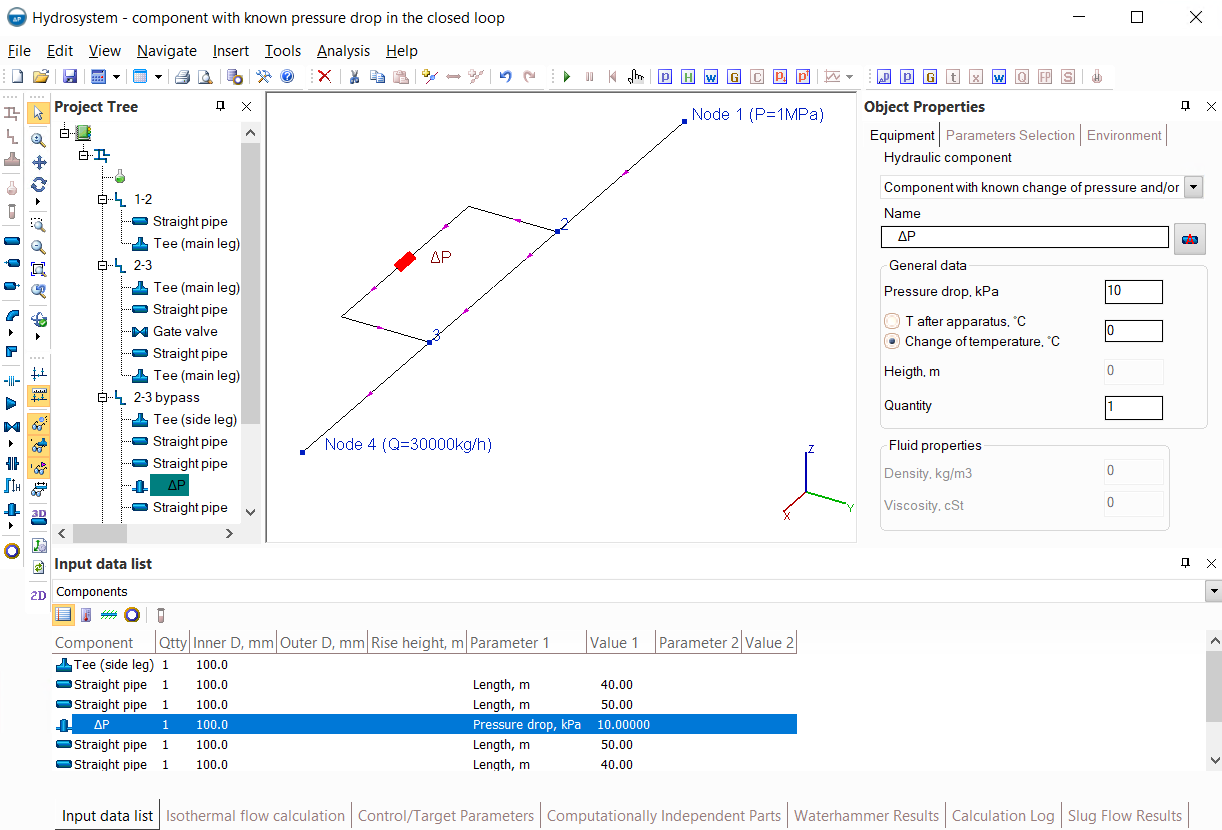
In this pipeline, the flow goes from node 1 to node 4 with a flow rate of 30000kg/h, and part of the flow goes straight (the "2-3" branch), and part bypassing the main flow-path (the "2-3 bypass" branch). There is a "Component with known change of pressure..." equal to 10 kPa in the bypass, and it is required to determine which part of the total flow rate (30000kg/h) will go through the main path via the branch "2-3", which bypasses (through this component with specified pressure drop via the branch "2-3 bypass"). To determine this, it is necessary to select such a flow distribution between the "2-3" and "2-3 bypass" branches, so their total resistances will be the same – in this example with these conditions, this is obtained at flowrates, respectively, about 25880 kg/h in the branch "2-3", about 4120 kg/h in the branch "2-3 bypass":

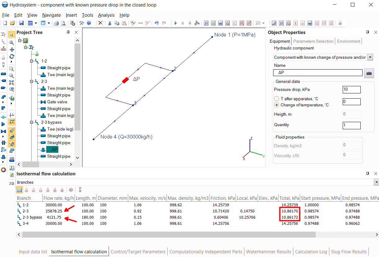
If, for example, the conditions of this calculation example would be so that the pressure drop on the "Component with known change of pressure..." is not 10, but, for example, 12kPa, then the calculation will give different values – slightly less fluid will be bypassed (since additional losses of 2kPa were added in this branch compared to the previous case):

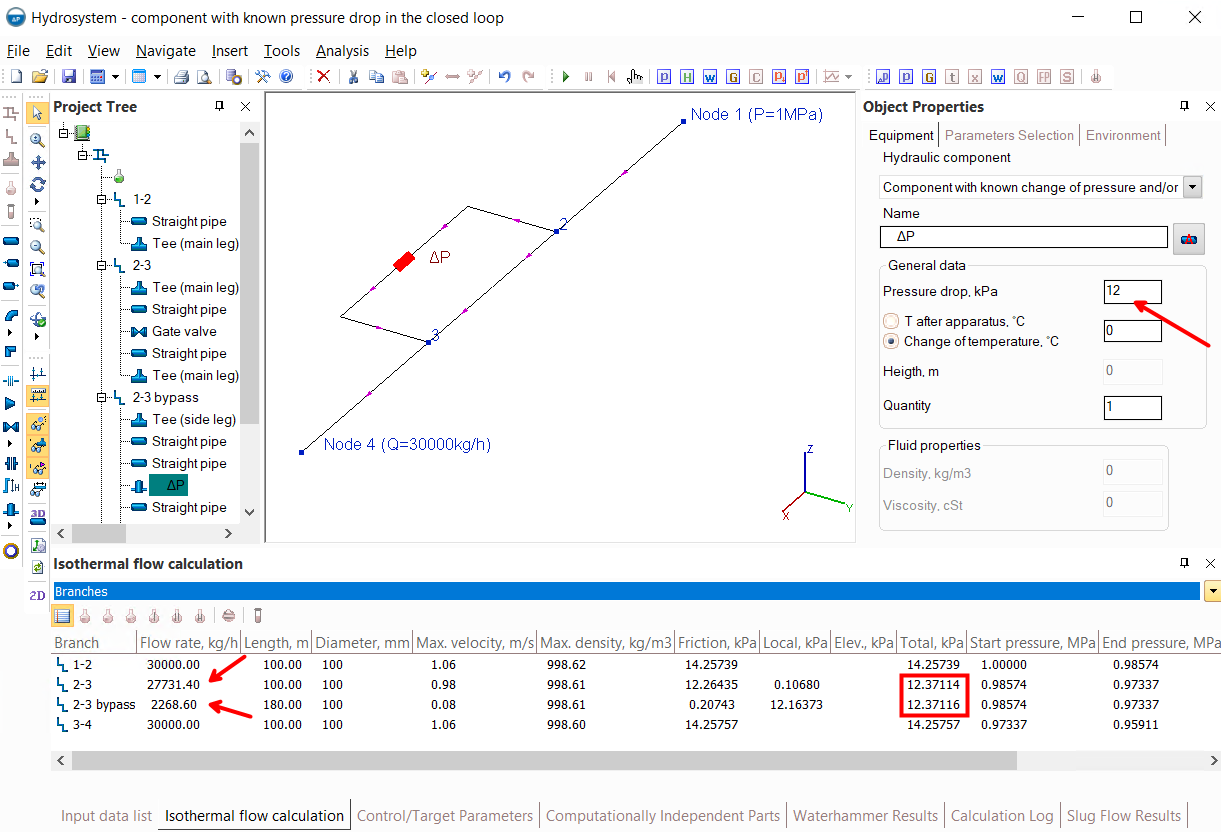
The key point here is that the solution exists in both cases (with 10 and 12kPa pressure drop) - that is, there is such a flow rates ratio in these two branches at which their total resistances are the same. And they must necessarily be the same, since both of these branches start at the same node 2 and end at the same node 3 - the difference between the pressure in node 2 and 3 will be the same regardless of "which side of the branches to look at" these nodes.

However, such a picture may not always take place. If the conditions of this calculation example would be so that the pressure drop on the "Component with known change of pressure..." is, for example, 20kPa, then the calculation will be interrupted with an error:

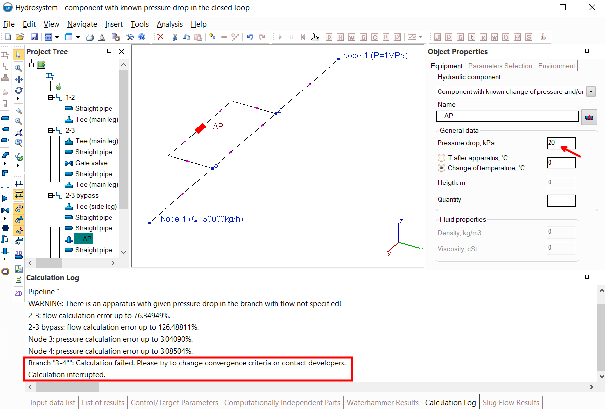
To understand why this is happening, it is most obvious to remove (or close) the "2-3 bypass" branch (with a resistance of 20kPa) and calculate how the flow will behave if it goes entirely through the branch "2-3" (without any bypass):

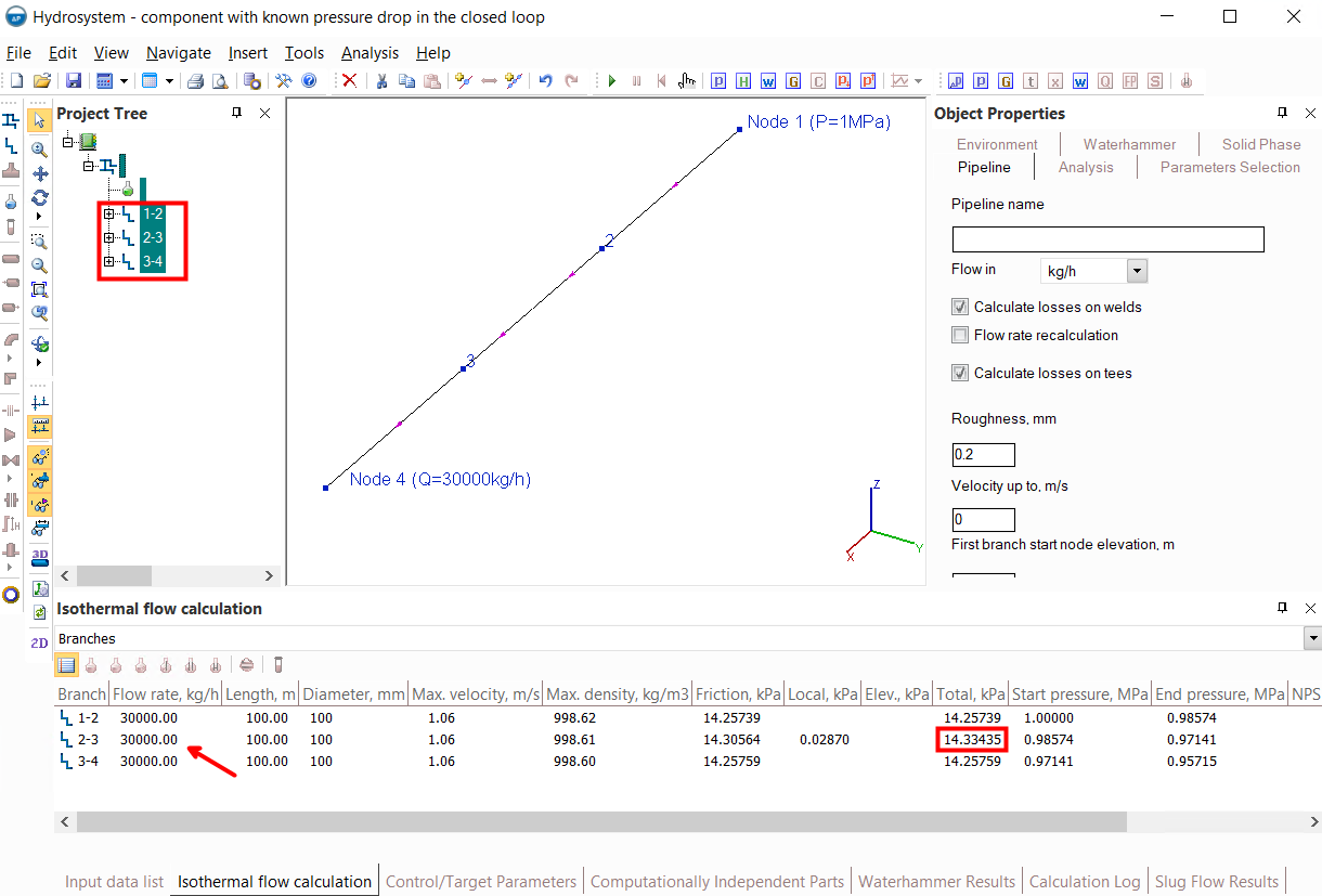
In this case, it turns out that even if the entire flow rate of 30000kg/h goes straight (and nothing goes in bypass), the total resistance of the branch "2-3" will be only about 14.33 kPa. That is, the difference between the pressure in node 2 and node 3, the maximum in the worst case for these conditions, can be 14.33kPa. But the "2-3 bypass" branch in the original pipeline also goes from the same node 2 to the same node 3 – that is, there should also be a total pressure drop of 14.33kPa in this branch. And, it's obvious, that it is physically impossible to loose altogether about 14.33kPa in the whole branch if only on the "Component with known change of pressure..." the pressure drop is already 20kPa (more than 14.33kPa) and there will still be some other losses on other elements of this branch. That is, with a pressure drop at a "Component with known change of pressure..." of 20 kPa, this calculation task simply have no solution. Or in other words, there is no such a flow distribution between these branches at which the pressure drop at a "Component with known change of pressure..." can be 20 kPa, as specified in the input data.

Moreover, it is important to clarify that this calculation task has no solution only at the specified total flow rate of 30000kg/h. If the flow rate is higher (for example, 50000kg/h), then a solution will be found in the case of a pressure drop at a "Component with known change of pressure..." of 20kPa (since the remaining resistances at such a flow rate will become larger):

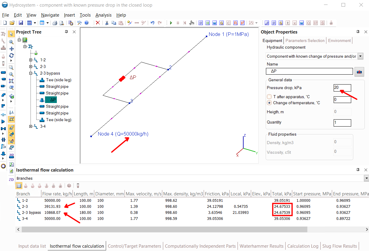
Thus, the existence of a solution of such a calculation task depends on many factors - flowrates, pressures, pipeline geometry, values of the pressure drop on the "Component with known change of pressure...", etc. In cases where a solution exists, the program finds it, but with some parameters, there simply may not be a solution.

However, regardless of whether or not there is a solution of this task, in any case, the "Component with known change of pressure..." does not reflect the behavior of real elements of piping systems, since it does not take into account the change in the hydraulic resistance of the element with the change of the fluid flow rate passing through it (the pressure drop on such an element is considered constant). Therefore, if there are "Components with known change of pressure..." in branches with unknown flow rates, the program shows the corresponding warning during calculation.

If you are sure that the "Component with known change of pressure..." correctly models what you want to model (for example, if the flow rate on branches with this component is controlled by flow regulator or it is indirectly known through the flow rates set in other branches), then this message can be ignored. Otherwise, it is recommended to use the element "Component with known loss coefficient" instead of "Component with known change of pressure...". The local loss coefficient in this case can be easily calculated through the pressure drop according to the well–known Weisbach equation Δp=ζρw2/2, where ρ and w are the density and velocity of the fluid, respectively, Δp is the pressure drop, ζ is the local loss coefficient. When using "Component with known loss coefficient", the above calculation task (as well as all similar tasks) will always have a solution, no matter what local loss coefficient is set (in the limit, with very large values of the local loss coefficient, the flow through it will tend to zero). Because for this element, the losses will be different, depending on the fluid flow rate passing through it. And returning to the example with the "2-3" and "2-3 bypass" branches, it will always be possible to find such a flow rates distribution between these branches so that their total resistances coincide.

The flow direction was changed in the branch containing apparatus or check valve or globe valve

If this message occurred during the calculation, it means that the input data for the calculation is set in such a way that the flow rate in the branch with the equipment or check valve as a result of the calculation turned out to be negative - that is, the flow goes in the opposite direction "backwards" through the apparatus/check valve.

If such a message is shown for a branch with a check valve, then the calculation results in this case will be incorrect, since in reality the check valve passes the fluid only in one direction, and when the pressure after the check valve is higher than before it, the valve closes, preventing the flow in the opposite direction. Unfortunately, this feature of the behavior of check valves is currently not taken into account in the calculations of steady-state flow (isothermal flow calculation, heat and hydraulic analysis or diameters calculation) in the Hydrosystem - the program considers such elements as working "both ways". Therefore, this message (if it occurred for a branch with a check valve) should be interpreted as the fact that the pipeline will not work in the specified mode. And it is necessary to change the flow parameters and/or characteristics of the pipeline so that the flow through the check valve goes in the "right" direction.

If such a message occurs for a branch with an apparatus (component with a known change of pressure), then the calculation results in this case will also be incorrect, since the pressure drop on the apparatus when the flow goes through it in the opposite direction is considered equal to its specified drop with the opposite sign, which is completely untrue. In this case, it should be remembered that it is not recommended to model such equipment as "Components with known change of pressure..." in branches with unknown flow rates in the first place, which is described in detail here. In such cases, it is recommended to use the element "Component with known loss coefficient" to model such equipment/device. The local loss coefficient in this case can be easily calculated through the pressure drop according to the well–known Weisbach equation Δp=ζρw2/2, where ρ and w are the density and velocity of the fluid, respectively, Δp is the pressure drop, ζ is the local loss coefficient.

Note: despite the above-mentioned flaws in the calculation algorithm of the Hydrosystem, it is difficult to call it really a "flaw" in the full sense of the word. The fact is that situations when a check valve closes or when the flow changes direction when moving through the equipment, in practice, are either "abnormal", or in principle should not occur at all and indicate errors in piping system design. In both cases, the calculation of this mode of operation of the pipeline system is not required, since it should not be operated in this mode anyway. Therefore, the diagnosis of the occurrence of these operating modes is more than sufficient in the design and verification calculations of piping systems.

The control parameter has reached the lower boundary

Such a message can be issued when calculating pipeline systems with parameters selection, if any flow parameter (most often pressure or flow rate) is regulated using an orifice, and a very small value of the orifice diameter/pipe diameter ratio is required to provide the required value of the selected parameter. The fact is that when selecting parameters for orifices, the program searches for a solution only in the range of values of the orifice diameter/pipe diameter ratio from 0.2 to 1. If the solution lies in the area below 0.2, then the practical expediency of searching for such a solution is not of a big sense for two main reasons - firstly, the accuracy of currently available methods for calculating the hydraulic resistance of orifices with such small openings is relatively low. And secondly, in the area of small diameter values, the resistance of the orifices is very "sensitive" even to the slightest changes in the diameter of its opening. That is, a change in the diameter of the orifice opening, even by fractions of millimeters, will cause a significant change in its hydraulic resistance. This can be clearly demonstrated by the following example:

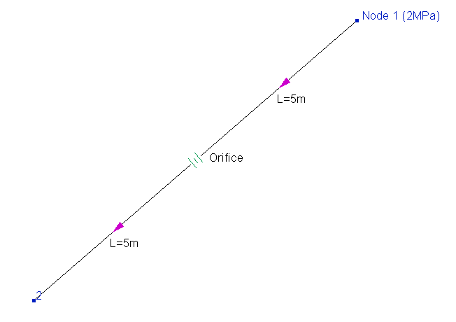
The pumped fluid in this pipeline is water (with a density of about 1000kg/m3), a pressure of 2MPa (abs.) is set in the initial node 1, the fluid is pumped with a flow rate of 30000kg/h (quite "typical" for a pipeline with such a diameter), the inner diameter of the pipeline is 100mm, its total length is 10m and in the middle the orifice is installed. If the diameter of the orifice opening is, for example, 18mm (the orifice diameter/pipe diameter ratio 18mm/100mm = 0.18), then its resistance will be about 1.5 MPa, and accordingly, the pressure at the end point of the pipeline will be about 2-1.5 = 0.5MPa abs. (the hydraulic resistance of the pipes before and after the orifice is negligible). If, for example, the diameter of the diaphragm opening is only half a millimeter smaller (i.e., 17.5mm), then its resistance will already be about 1.67 MPa (and the final pressure will be about 0.33 MPa abs.). Therefore, if this orifice is used to adjust, for example, the pressure at the end of the pipe 0.4MPa abs., then, accordingly, an orifice with an opening diameter somewhere between 17.5 and 18mm is required. As you might guess, manufacturing an orifice with a diameter exactly equal to the required one will be extremely problematic in practice. And the "inaccurate" manufacture of the orifice in this case is unacceptable, since it is worth making a mistake by just a fraction of a millimeter and such an orifice will adjust the 'wrong' pressure.

Thus, the calculation of the orifice diameter in the case of small values is not of practical interest. That is why, if, when calculating with parameters selection, the value of the orifice diameter/pipe diameter ratio 'drops' into the range of values less than 0.2, the program interrupts the calculation with the error indicated above. In such cases, it is recommended to use any other control devices more suitable for these cases - for example, control valves, for which in most cases it is possible to select such a valve with which maintaining the required flow/pressure value of the fluid will not cause problems.

Unknown error, calculation does not converge, internal error, etc.

Unfortunately, not all errors that occur in the calculation can be easily diagnosed. Some errors in the input data or features of the piping model can lead to problems in the calculation for which it is difficult to find an unambiguous cause. In addition, they may have several different causes, or they may be the result of some completely different problem. In all cases where it is impossible to determine exactly what caused the problem in the calculation, the program shows the "abstract" messages about an internal error, an unknown error, a non-convergence of calculation, etc. If such errors occur, it is recommended to check all the input data and if no visible errors/typos are found in the input data, then contact the technical support of the program.