Additional functions of the program
Plotting a piezometric profile
The results of pipeline calculations can be presented in the form of a so-called piezometric profile graph, showing the change in the pressure of the pumped liquid along the pipeline. It is especially convenient to use a piezometric graph for heating networks and other pipelines of circulating cycles, in which the working liquid is supplied through a feed pipeline to the consumer and returns through a return pipeline, which has approximately the same configuration as the supplying one, since to construct such a graph it is not necessary to model both parts (feed and return) of the pipeline in the Hydrosystem. It is enough to model only the feed line, and the graph for the return line can be automatically generated on the basis of the feed line geometry.
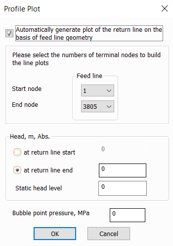
To plot a piezometric graph, it is necessary to calculate the steady flow (isothermal flow analysis, diameters calculation or heat and hydraulic calculation) of the feed pipeline, and then select the menu item "File - Profile Plot...". A window will appear in which you will need to specify:
the way to plot the graph - from which node of the pipeline to which it is necessary to form a piezometric graph. Usually, the source node where the heating plant is located is selected as the start node, and either the most distant consumer or the most "hydraulically remote" one (along the way to which the pressure losses due to friction and local resistance are the highest) is selected as the end node. However, if necessary, a graph can be plotted between any other nodes of the pipeline;
the head either at the beginning or at the end of the return line - this head value serves as a reference point relative to which the calculation of the return line of the pipeline will be performed. By default, it is assumed that the return line pipeline has exactly the same configuration as the feed line (even if they do not exactly match each other, minor discrepancies can be neglected), and the pressure losses in it are assumed to be the same as in the feed one (except for hydrostatic losses, which are assumed to be the same, but with the opposite sign). You can specify the pressure at the end of the return pipe, if it is known with what pressure the fluid should be supplied to the suction of the circulation pumps and it is necessary to determine the permissible losses at the consumer, or at the beginning of the return pipe, if, on the contrary, the losses at the consumer are known (and, as a consequence, the pressure at the outlet of the consumer) and it is necessary to determine whit what pressure the fluid will reach the heating plant;
static head level - shows the pressure in the event of pumping stop and is plotted on the piezometric graph as a horizontal line (it is not necessary to specify it);
bubble point pressure - this field must be filled only if the product properties are specified explicitly and the saturated vapor pressure is not specified. When modeling the pumped product using thermodynamic libraries, there is no need to specify the saturated vapor pressure separately, since the libraries can calculate it automatically.
By default, the graph for the return pipeline is generated automatically, based on the assumption that its geometry coincides with the geometry of the feed line. However, if necessary, if the calculated pipeline model includes not only the feed line, but also the return line, you can build a graph for the return pipeline based on the calculated data. To do this, turn off the "Automatically generate plot of the return line on the basis of feed line geometry" option and enter the number of the start and end nodes of the return line (note that this function will only work if the number of nodes in the graph for the feed and return pipelines is the same). In this case, you do not need to specify the pressure at the start/end of the return pipe.
After entering all the data and clicking the "OK" button, the program will offer to select possible paths for constructing a piezometric graph. For pipelines containing loops, there may be several such paths. When clicking the "Show" button, the selected path will be displayed in blue on the diagram:
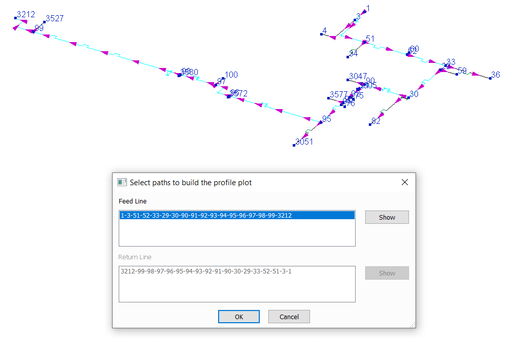
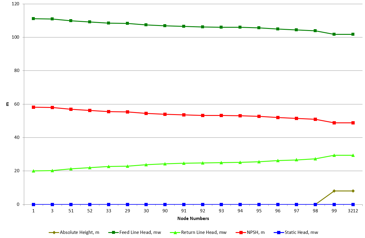
Select the path you are interested in and confirm it by pressing the "OK" button. After that, a standard window will open in which you will need to specify the name of the data file (in .csv format) for plotting the piezometric graph. And after saving this file, if Microsoft Excel is installed on this PC, the corresponding Excel file will be automatically generated (in the same directory with the same name as the csv data file), on one sheet of which there will be a table with data, on the other - a diagram displaying the following curves:
pipeline height curve (absolute height – Z) of the pipeline;
static head line (pressure in the system when pumping stops);
full head curves (but without the acceleration head component) for the feed and return pipes – when constructing these curves, the piezometric pressure P/(g*ρ) is plotted along the ordinate axis from the pipeline height curve, where P is the pressure, ρ is the density of the liquid at the current temperature and pressure in pipe, g is the acceleration due to gravity. In other words, the curves are given by the formula Z+P/(g*ρ);
NPSH curve for a feed pipe, determined by the formula Z+(P-Psat)/(g*ρ), where Psat is the bubble point pressure of the liquid at the current temperature in pipe.
The program provides a function for combining adjacent straight pipe sections with the same properties (diameters, roughness, location parameters, etc.) and the same direction in space. When combining, several consecutive sections are transformed into one straight pipe section with a length equal to the sum of the lengths of the original sections. Such a function may be required, for example, for more convenient work with pipelines imported from other programs and files (pcf, AVEVA, etc.), since often when importing data, each small detail of the pipeline (like flanges, gaskets between them, etc.) is imported as a separate piping section with a microscopic length. Using this command, you can combine such sections.
To merge sections, select either
the branch in which you want to merge sections, or the entire pipeline
(if you want to merge sections of all branches) and click the
 button of the Edit toolbar or
use the option "Integrate Pipes" in the Edit menu or the context
menu called by right-clicking on the element in the project tree.
button of the Edit toolbar or
use the option "Integrate Pipes" in the Edit menu or the context
menu called by right-clicking on the element in the project tree.
The Hydrosystem has a function for automatically recalculating the geometric characteristics of various piping components according to their location on the graphic diagram. These include:
bends and elbows angles and elevation differences;
reducers elevation differences;
lengths and elevation differences of straight pipes with the "Loop closing pipe" option enabled.
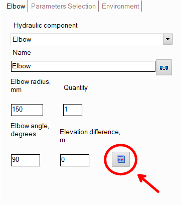
The point is that the parameters specified above are initially set manually by the user in the input data, and their values may not correspond to the location of these elements on the graphic view (for example, the user has modeled the elbow so that it "turns" upward, but forgot to set the elevation difference for it). The "recalc by graphics" option eliminates these discrepancies by calculating the geometric parameters of bends, reducers, etc. according to their graphic location and automatically writing them into the input data for calculating these elements. To run recalculation by graphics for all pipeline elements, use the "Tools - Recalc by Graphics" menu option. If recalculation by graphics needs to be performed for a single pipeline element, select it and use the corresponding button in the Object Properties Window:
Please note that the "Recalc by graphics" function will be available only if the "Scaled graphic view" and "Show all components" options are enabled in the pipeline graphic view options (on the View Options toolbar); in addition, the "Precise graphic representation of scaled view" option must be enabled in the program settings. Otherwise, the graphic display of the pipeline is conditional, and the location of elements on the graph may not exactly correspond to their actual location in the pipeline. Because of this, recalculation by graphics may give incorrect results, so it is not available in these modes.
In addition, in the program settings you can enable the option "Recalculate elevations and angles on graphic before every analysis" - if it is turned on before each calculation the program will automatically recalculate the elevation differences on all pipeline elements, bend angles, etc. and store/correct them in the input data.
Recalculation of pipes projections
When you run the "Tools - Recalc layout" menu option, all user-specified directions of pipes and other pipeline elements will be ignored, and the layout of elements on the piping diagram will be recalculated. This option is obsolete and is generally not used in the latest versions of Hydrosystem. Its use was relevant in very old versions of Hydrosystem, which did not yet have the ability to specify the spatial arrangement of elements (in the form of projections of their lengths on the X, Y and Z coordinate axes). Using this option, it was possible to "redraw" the pipeline diagram in such a way as to minimize overlapping of pipeline elements. In modern realities, this option is of no particular practical use.
Elevation mismatches correction
The Hydrosystem has a special function for automatic search and elimination of inaccuracies in elevation differences on elements located in closed loops. The fact is that the values of elevation differences on elements and vertical projections of pipe sections are very important in hydraulic calculations (especially for flows containing a liquid phase), since hydrostatic differences on elements (whose contribution to the total resistance is usually very large for liquids) depend on their values. Therefore, errors and inaccuracies in vertical projections and elevation differences of pipeline elements can cause a significant calculation error. And if these inaccuracies are contained in closed loops of pipelines, this can also cause problems with the convergence of calculations of such pipelines.
As a clear example of such errors, the model of a pipeline is given below, in which the flow follows different paths from node 1 to node 6. And as is easy to see, somewhere for one (or several) pipe sections of the closed loop there is an error in the values of lengths/height differences, due to which a "gap" in the pipeline model occurs at node 5:
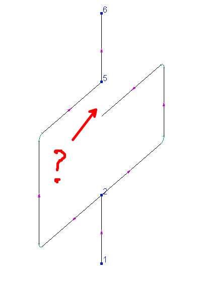
Mathematically, this means that the flow needs to overcome one height (and spend one amount of energy on this rise) in order to rise from node 2 to node 5 along the "left shoulder" of the pipeline, and completely different height along the "right shoulder". If the value of this inaccuracy is small, then this will cause only a small error in the calculation of the flow distribution between the left and right "shoulders" (the calculated flow rate along the right "shoulder" will be greater than it should be). But if this inaccuracy is large enough, it can cause fundamental changes in the picture of what is happening in the pipeline (for example, in the calculation it may turn out that the flow along the left shoulder goes "backwards", being unable to overcome such a difference in height, and a kind of "recirculation" occurs) to the point that the problem will have no solutions at all.
Unfortunately, it is impossible to clearly define where the boundary lies between "small" and "large enough" (to cause problems) inaccuracy of height differences. This depends on many factors (on the values of flow rates and pressures in the system, on the values of other resistances of branches, etc.), and if in one pipeline an inaccuracy in height of 20-30 cm will cause only a small calculation error, then for another piping model such an inaccuracy can be critical. Therefore, just in case, when modeling a pipeline in the program, it is better to pay special attention to specifying vertical projections of pipe sections and elevation differences on bends and reducers located in pipelines with closed loops.
However, if there is an inaccuracy somewhere in the pipeline that may cause calculation convergence problems, when attempting to calculate such a pipeline, the program will show a corresponding message about this in the calculation log, indicating on the diagram the place (in blue) where the inaccuracy in heights is found, and its magnitude:
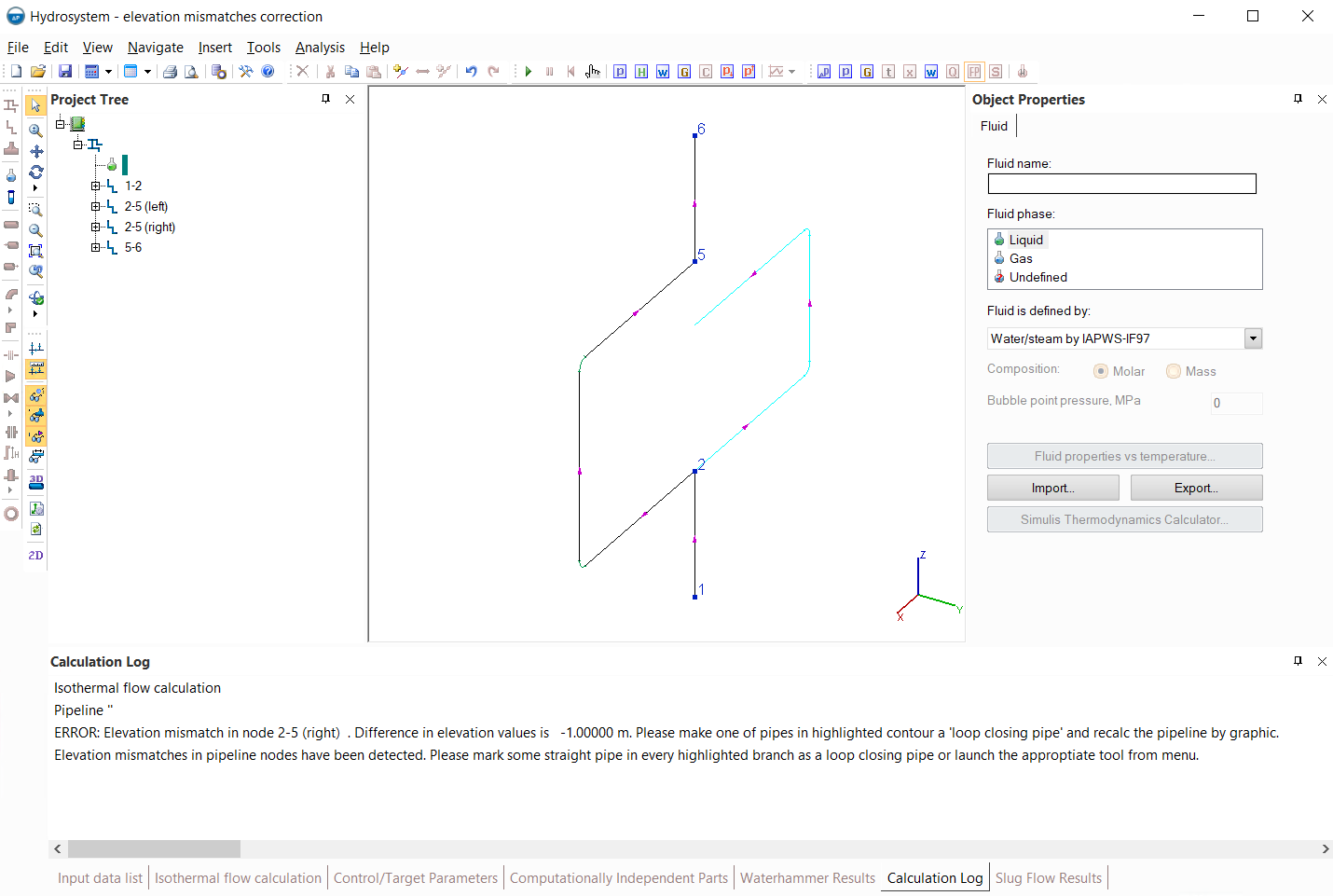
It is important to understand that the program cannot reliably determine on which element of the closed loop the error was made - in the example above, this error can be on the "left" vertical pipe section, as well as on the "right" one (as well as on the horizontal sections of the loop - for example, they can actually be inclined and the user forgot to set the projections on the Z axis for them). Only the user can unambiguously determine where the error is by checking the input data for all elements. Therefore, the message in the calculation log that an elevation mismatch is in some specific branch/node should not be taken literally (it says that this mismatch is found in this branch, but the inaccuracy in input data that caused this mismatch may be in some other place in this closed loop) - it should be understood as a signal that there is an inaccuracy somewhere in this closed loop. And in order to be able to perform the pipeline calculation, this inaccuracy must be corrected - for this, you can use a special service for correction of elevations mismatches by running the corresponding command in the "Tools" menu. This function works as follows: for all pipeline elements, "Recalculation by graphics" (for more details on that, see here) is performed and for each closed loop in the pipeline, one of the pipe sections will be randomly (!) assigned as a "loop closing pipe" so that the lengths of its projections on the coordinate axes are recalculated to eliminate the inaccuracy in the closed loop. After eliminating the mismatches, the pipeline calculation will be performed. However, please note that the loop closing pipe in this algorithm is selected randomly. As already mentioned above, the program "does not know" where exactly the error is in the closed loop, so it is possible that this error will be corrected in a completely different pipeline element from where it was made. So this service is recommended to be used only in the most extreme cases; it is advisable to find and eliminate such errors yourself, having checked the correctness of the input of data on the pipeline geometry into the program.
Please note that the "Correct Elevation Mismatches" function will be available only if the "Scaled graphic view" and "Show all components" options are enabled in the pipeline graphic view options (on the View Options toolbar); in addition, the "Precise graphic representation of scaled view" option must be enabled in the program settings. Otherwise, the graphic display of the pipeline is conditional, and the location of elements on the graph may not exactly correspond to their actual location in the pipeline. Because of this, recalculation by graphics may give incorrect results, which is why the elevation mismatches correction service is not available in these modes.
Topological analysis of the pipeline model
The Hydrosystem has a special service that allows you to analyze the "coherence" of the calculated pipeline model and diagnose calculation-independent fragments in it. This service is useful in cases where it is interesting to understand how the pipeline is calculated (which of its fragments are considered and calculated independently of each other), and also if during the pipeline calculation the errors "Pipeline contains unconnected parts..." or "The system breaks down into disconnected areas..." occur, related to errors in the modeling of the pipeline or insufficient data for the calculation. The operation of this service is described in detail here.
The Hydrosystem provides a function for connecting any two pipeline nodes with a new branch. To launch this function, use the menu item "Tools - Connect Nodes...":
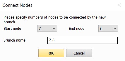
In the window that appears, you need to specify which nodes need to be connected and optionally specify the name of the branch connecting them. After this, a new branch will be added to the pipeline connecting these nodes, which will contain a straight pipe with a length and direction corresponding to the distance between these nodes (note that the diameter of the added branch will not be specified - if necessary, you can then specify it manually). This command is particularly convenient for combining unconnected fragments in a pipeline.
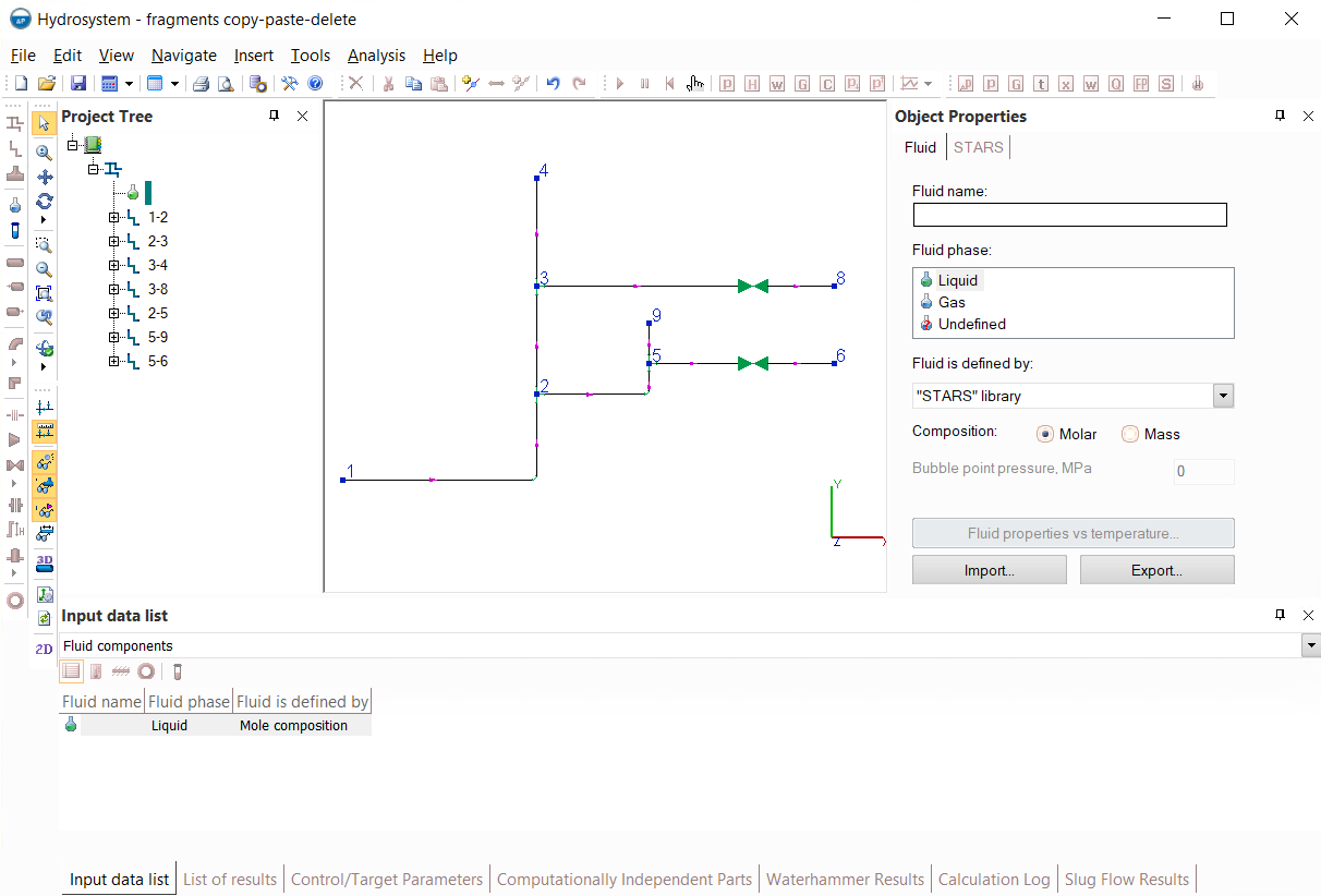
The Hydrosystem provides the ability to copy/paste both separate branches and piping components, multiple branches/components and entire pipeline fragments consisting of several components/branches. Let's consider this using the example of a pipeline shown in the figure below. In this pipeline, it is necessary to copy the fragment from node 3 to node 8 and paste it so that it exits node 4 and goes to a new pipeline node (for example, number 10):
This can be done in several different ways:
Method #1 - copying several elements of a branch. To do this, you need to:
Add another branch to the pipeline and set node 4 as its starting point and node 10 as its ending point;
Select all components from the "3-8" branch (except the tee) in the graphics window or in the project tree - to select several elements, select the first of them and then, pressing and holding the Shift key, select the last one (if you need to select not all, but only some of the elements of this branch, after selecting the first element, press and hold the Ctrl key and click on all the elements that need to be selected in turn);
Select the Copy command of the Edit toolbar or the Edit menu (or simply press Ctrl+C on the keyboard);
Select the branch added in step 1 from node 4 to node 10 in the project tree and select the Paste command of the Edit toolbar or the Edit menu (or simply press Ctrl+V on the keyboard).
Method #2 - copying the entire branch. To do this, you need to:
Select the original branch "3-8" of the pipeline in the project tree and copy it by selecting the Copy command of the Edit toolbar or the Edit menu (or simply press Ctrl+C on the keyboard);
Paste the copied branch by selecting the Paste command of the Edit toolbar or the Edit menu (or simply press Ctrl+V on the keyboard). Note that the pasted branch in the project tree will have the same name as the original one, but the numbers of the start and end nodes will be completely different - not related to the rest of the pipeline. Therefore, the next step is to:
Change for the inserted branch its start node to node 4 and its end node to node 10.
Please note that you can also copy/paste multiple branches the same way by selecting several branches in the project tree using Ctrl or Shift keys.
Method #3 - copying a pipeline fragment from one node to another. For more clarity, let's consider this using the example of copying a fragment from node 2 to node 6 and inserting it into node 4 (so that this fragment consists of not one, but two branches). Unlike the case of copying elements between nodes 3 and 8 discussed above, here copying a separate branch or components of a branch will not be entirely convenient, since you need to copy several elements from different branches. Therefore, in this case, it is more convenient to use copying a pipeline fragment from one node to another. To do this, you need to:
Select node 2 on the piping diagram, press and hold the Shift key, then select node 6 on the diagram;
Select the Copy command of the Edit toolbar or the Edit menu (or simply press Ctrl+C on the keyboard);
Select node 4 on the diagram into which you need to paste the copied segment;
Select the Paste command of the Edit toolbar or the Edit menu (or simply press Ctrl+V on the keyboard) - the copied branches will be pasted into the project tree under the same names as the original branches, but with appropriate node numbers (the program will assign the first unused numbers to the new nodes) and no further editing will be required.
Each of the methods may be more convenient than others in certain cases, so it is recommended to use them depending on the situation.
Similarly, you can cut or delete fragments of pipelines.
Also Hydrosystem provides the ability to change the parameters of branches or individual piping components in groups. To do this, they must be selected in the project tree or in other program windows, after which the Object Properties window will display the parameters that can be changed for them simultaneously. For branches, these will be the values of diameters, flow rates, temperatures, roughness and other characteristics, for piping components - location parameters, thermal insulation, etc.
To select several elements (branches or piping components), select the first of them and then, pressing and holding the Shift key, select the last one (if you need to select not all, but only some of the elements, after selecting the first, press and hold the Ctrl key and click on all the elements that need to be selected in turn).