Boundary conditions of hydraulic calculation
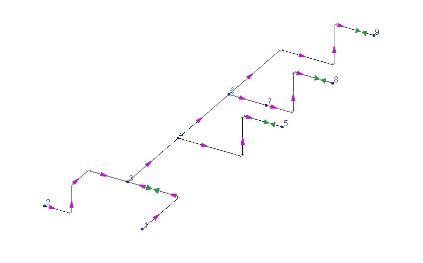
The formulation of the hydraulic (isothermal or thermal) calculation task may be different depending on what is the purpose of the calculation. And the purposes of the calculation in turn may be completely different - calculation of the flow capacity and flow distribution, calculation of upstream pressure and downstream pressure, etc. As an example, let's consider the pipeline system below, consisting of the following set of branches * (the division of the pipeline into branches is described in detail here), the geometric configuration of which (including the diameter values) is completely known:
| Branch | Starting node | End node |
Branch A |
1 |
3 |
Branch B |
2 |
3 |
Branch C |
3 |
4 |
Branch D |
4 |
5 |
Branch E |
4 |
6 |
Branch F |
6 |
7 |
Branch G |
7 |
8 |
Branch H |
6 |
9 |
For greater clarity, let us consider a case in which there are no inflows/outflows of flow in the intermediate nodes ** . The hydraulic calculation of this pipeline is reduced to solving the following system of equations:
P1 - P3 = f(QA);
P2 - P3 = f(QB);
P3 - P4 = f(QC);
P4 - P5 = f(QD);
P4 - P6 = f(QE);
P6 - P7 = f(QF);
P7 - P8 = f(QG);
P6 - P9 = f(QH);
QA + QB - QC = 0;
QC - QD - QE = 0;
QE - QF - QH = 0;
QF - QG = 0
where Pi is the pressure in the corresponding node i, QN is the flow rate in branch N of the pipeline.
This system consists of 12 equations: the first 8 of them describe the relationship between pressure losses in each of the 8 branches of this pipeline and the fluid flow rates in these branches (for information on how pressure losses depend on flow rates, see here), the remaining 4 describe the balance of flow rates in the intermediate nodes of the pipeline (the sum of the flow rates of the incoming flows into a node is equal to the sum of the outgoing flows). As you can see, there are only 17 variables in this system - the pressure values in 9 nodes and flow rates in 8 branches of the pipeline. Therefore, in order for this system of equations to be exactly determined and have a single solution, the values of 5 of its independent (!) variables should be known. Thus, the number of unknowns in the system of equations will be equal to the number of equations to be solved. The variables of the system, the values of which are taken as known in the calculation, are called boundary conditions of the hydraulic calculation. In Hydrosystem, the boundary conditions are specified by specifying the known pressures and/or flowrates values for the corresponding branches and nodes of the pipeline in the input data. The pressures and flowrates in all other nodes/branches of the pipeline are considered unknown and are not specified in the initial data - they will be determined by solving the system of equations described above.
Depending on which flow parameters in the hydraulic calculation are assumed to be known (i.e., which boundary conditions are specified), several various hydraulic calculation task are distinguished, among which the most common in practice are the following:
verification "downstream" calculation (or calculation of pressure losses along the flow path) - the boundary conditions for such a calculation are known pressure values at all initial points of the pipeline (at nodes 1 and 2 for the example above) and known fluid flowrates in all final branches of the pipeline (for the example above, these are branches D, G and H). In this case, there is no need to specify the pressures and flowrates in all other nodes/branches of the pipeline - they will be determined when solving the system of equations described above. This formulation of the calculation task is used in cases where the fluid pressure at the beginning of the pipeline is known (for example, the fluid is pumped by a pump whose head is known, or the fluid is supplied from a tank with a known liquid level, etc.) and it is necessary to determine how much the pressure will drop at each of the final points of the pipeline when pumping a certain (specified) fluid flow rate;
verification "upstream" calculation (or calculation of pressure losses against the flow direction, or "reverse" calculation) - the boundary conditions for such a calculation are the known pressure values at all end points of the pipeline (at nodes 5, 8 and 9 for the example above) and the known fluid flowrates in all initial branches of the pipeline (for the example above, these are branches A and B). In this case, there is no need to specify the pressures and flow rates at all other nodes/branches of the pipeline - they will be determined when solving the system of equations described above. This formulation of the calculation task is used in cases where it is necessary for the fluid to reach the consumer/consumers with a certain (known) pressure and it is necessary to determine what the pressure at the beginning of the pipeline should be for this (for example, in order to size a pump based on this pressure) when pumping a certain (specified) fluid flow rate;
calculation of pipeline flow capacity (or flow rate calculation) - the boundary conditions for such a calculation are the known pressure values at all initial and final points of the pipeline (at nodes 1, 2, 5, 8 and 9 for the example above). The pressures at all other nodes of the pipeline, as well as the flow rates in all branches of the pipeline, do not need to be specified in this case - they will be determined when solving the system of equations described above. This formulation of the calculation task is used when the pressures at the boundaries of the pipeline are fixed and it is necessary to determine what flowrate the pipeline can "pass through" (and how the flows will be distributed) with a given pressure difference.
There also can be other hydraulic calculation tasks options - for example, when the flow rates are known for some of the initial and final points of the pipeline, and the pressures for others, or when the pressures, for some reason, are known at some intermediate points, etc. Such tasks in the Hydrosystem can also be solved by setting the appropriate boundary conditions for the calculation, however, in practice such tasks are not of a big interest and therefore, extremely rare.
How you shouldn't specify boundary conditions for hydraulic calculations
As mentioned above, to perform hydraulic calculation the system of equations must be exactly determined - that is, the number of equations must be equal to the number of unknowns in the system. To ensure that the system is determined, it is enough to follow the following rule - for each initial and final point of the pipeline, it is necessary to specify either the pressure or the flow rate (for the above example of the pipeline, which has 2 initial and 3 final points, in this case the values of 5 variables are specified - exactly as many as are necessary to "close" the given system). If at least for one initial or final point of the pipeline neither the pressure nor the flow rate is specified, then such a system is underdetermined (that is, the number of unknowns in it is greater than the number of equations, and it will have infinitely many solutions). This is easy to see if, for example, for the above example of the pipeline system, neither the pressure at node 1 nor the flow rate in branch A (starting at this node) are specified as boundary conditions. In this case , it will not be possible to solve the first equation "P1 - P3 = f(QA)" in this system (even if it is possible to uniquely determine the value of P3 by solving the remaining equations in the system), since this equation will contain two unknowns *** . In other words, the flow rate from a node and the pressure at this node are interrelated quantities (the relationship between which for this node is described by the equation "P1 - P3 = f(QA)", for other nodes - by similar equations). If the pressure at node 1 is known, then the value of the flow rate in branch A is "pre-determined" by the value of this pressure (the higher the pressure at the node, the greater the flow rate will be). And vice versa, if the flow rate at branch A is known, then its value determines what the pressure at the node will be (the higher the flow rate, the greater the pressure will be). The same applies to the end nodes of the pipeline - the flow rate going to the end node is directly related (through the corresponding pressure loss equation) to the pressure at this node. Therefore, in order for the calculated system to have one unique solution, for each starting and ending point of the pipeline, one of the quantities (pressure or flow rate) must be known and specified in the initial data for the calculation, the other is unknown and not specified.
If, on the contrary, for at least one initial or final point of the pipeline the values of both pressure and flow are specified, then in this case the system becomes overdetermined (but only provided that for all other initial and final points either pressure or flow is specified, otherwise, as described above, the system will still be underdetermined). In such a system the number of unknowns is less than the number of equations, and usually such systems are inconsistent (since equations contradict each other) and have no solutions. That is, such a formulation of the hydraulic calculation task, when for the same initial/final point of the pipeline both the value of pressure and flowrate are known, is incorrect - these values, as already mentioned above, are dependent on each other, and when both of them are specified, their values may contradict each other. To avoid such incorrect task formulations, there is a special rule in the program - the specified value of pressure in a node has a higher priority compared to the value of flow rate in the branch adjacent to it. Therefore, if both pressure and flow rate are specified for some initial or final point of the pipeline, the entered flow rate value is ignored and recalculated as it will be at the specified pressure in the node. As mentioned above, the flow rate in this case is unambiguously determined by the pressure value with the corresponding pressure losses equation.
From all of the above, several important facts logically follow:
only variables that are independent of each other must be selected as boundary conditions for hydraulic calculations, otherwise (if you specify interrelated parameters as boundary conditions) their values may contradict each other, due to which some of these parameters (flow rates) will be discarded and recalculated when solving the system of equations (that is, they will not be perceived as boundary conditions);
providing both the specified pressure value and the desired flow rate at the initial or final point of the pipeline is impossible "in itself". For example, if the pressure value is fixed at the final point of the pipeline, the flow rate to this point will not "magically' become the one "needed by the designer". As they say, "the flow is not a trained puppy" - it is distributed in the pipeline based on the resistance of the pipeline branches and the pressure values at the points from/to which it goes (and not based on piping engineer wishes). Therefore, the only way to simultaneously provide both the specified pressure and the required flow rate at the initial/final point of the pipeline is to regulate the flow rate using flow control valves or other control devices;
setting the pressure in intermediate pipeline nodes may result in an imbalance of flows in this node (i.e., the sum of the flows entering this node will not be equal to the sum of the outgoing flows). This is due to the fact that, as mentioned above, the pressure value in a node has a higher priority in the calculation than the flowrate value. Thus, if a pressure is set in an intermediate node, the flows in the branches adjacent to this node will be recalculated based on this pressure value, as a result of which the sum of the inflows/outflows in the node may not be equal to zero. Therefore, it is not recommended to specify pressures in intermediate pipeline nodes during calculations, unless this is justified by the specifics of the calculation task being solved (for example, this may occur if several branches end in some intermediate node, but none begin, or vice versa, several branches begin, but none end. For such nodes, pressures are specified in some cases, since from the point of view of calculation, such a node is considered, respectively, as a consumer node or a source node).
Please note that only pressures or flowrates at the boundaries of the pipeline system (i.e., at the initial and final points) can be specified as boundary conditions for the hydraulic calculation. The flows in intermediate pipeline branches (that are not initial or final) specified in the initial data are considered only as initial approximations for the calculation and cannot be boundary conditions for the hydraulic calculation. Moreover, if, for example, we the pipelines with closed loops (pipelines with rings, recycles, etc.) is considered, the flowrates in the intermediate branches of such a pipeline are almost always recalculated at the calculation. This is due to the fact that the distribution of flows in the branches of closed loops is determined exclusively by the geometry (resistances) of the elements included in these branches, and thus the flows in such branches are determined automatically when solving the system of equations describing the pipeline. Therefore, as already mentioned above, the flow rate in the branches of a closed pipeline will not be established as required "by itself" - in order for the flow rate in such branches to be equal to the required one, it is necessary to regulate it using flow control valves or other control devices.
Boundary conditions for the pipeline diameters calculation
Unlike the isothermal flow analysis and heat and hydraulic calculation of a pipeline, at which the piping diameters values are assumed to be known, at the diameters calculation the diameters of the pipeline branches are unknown quantities that need to be determined. Since pressure losses in a pipeline also depend on the diameter values, new variables (the diameter values of each branch) are added to the system of equations for the above example of a pipeline in the design calculation, and this system is rewritten as follows:
P1 - P3 = f(QA, DA);
P2 - P3 = f(QB, DB);
P3 - P4 = f(QC, DC);
P4 - P5 = f(QD, DD);
P4 - P6 = f(QE, DE);
P6 - P7 = f(QF, DF);
P7 - P8 = f(QG, DG);
P6 - P9 = f(QH, DH);
QA + QB - QC = 0;
QC - QD - QE = 0;
QE - QF - QH = 0;
QF - QG = 0
where Pi is the pressure in the corresponding node i, QN is the flow rate in branch N of the pipeline, DN is the diameter of branch N.
This system still has 12 equations, but this time it has 25 variables - pressure values at 9 nodes, flow rates at 8 branches and diameters of 8 pipeline branches. Therefore, in order for this system of equations to be exactly determined and have a single solution, the values of 13 of these variables should be known. Usually, the diameters calculation task is formulated in such a way that it is known with what pressure the fluid is supplied to the pipeline (at the starting points), with what pressure the fluid should reach each the consumers (end points) and what fluid flow rate should be pumped in each of the pipeline branches. Therefore, the boundary conditions of the diameters calculation are always the pressures at all starting and ending points of the pipeline and the fluid flow rates in all pipeline branches without exception (for the pipeline above, these will be the pressures at 2 starting, 3 ending nodes and flow rates in 8 branches - a total of 13 variables). The pressures in the intermediate nodes and the diameters of the pipeline branches are considered unknown and are not specified in the initial data - they will be determined when solving the system of equations described above.
It is important to understand that if at least one of the above boundary conditions is not specified, this makes the system of equations being solved underdetermined. For example, if for the above pipeline model the pressure at node 9 is not specified in the diameters calculation, this makes the value of the diameter of branch H undefined - since for this branch it is possible to select "any" (within reasonable limits) diameter value and with this value some pressure value at node 9 will be obtained (that is, the system will have an infinite set of solutions). In other words, what value of the diameter of a given branch should be taken depends on what pressure is required to be obtained at the end of this branch (similarly for other nodes/branches of the pipeline).
Theoretically, the calculation of diameters can also have such a formulization, in which the pressures are known not at the initial/final nodes of the system, but at some intermediate points of the pipeline. However, such calculation tasks are of no practical interest, so they are not considered in the calculations in the Hydrosystem. The only exception is cases in which several branches end in some intermediate node, but none begin, or vice versa, several branches begin, but none end. In this case, in such a node, it is necessary to specify the pressure (to be able to calculate diameters), since from the point of view of the diameters calculation, such a node is considered, respectively, as a consumer node or a source node.
Please note that, unlike isothermal flow analysis and heat and hydraulic calculation, in which the flow rates in intermediate pipeline branches are considered only as initial approximations for the calculation and nothing more, in the dcalculation, the flow rates in all branches are boundary conditions for the calculation, so they must be specified in the initial data for all branches, including intermediate ones. This is due to the fact that for some types of pipeline schemes, the flow rates in intermediate branches are not uniquely determined by the flow rates in the initial and final pipeline branches. Below is an example of such a scheme:
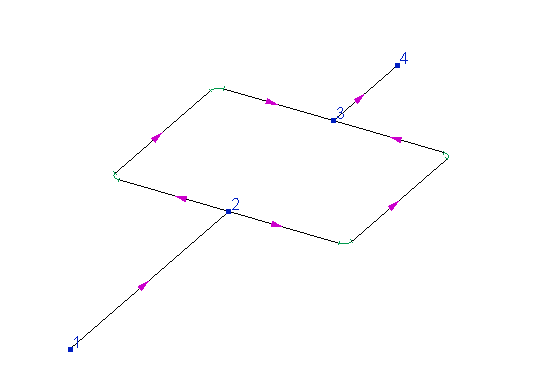
In this pipeline, the flow can be divided at node 2 into two, for example, equal parts, or the larger part of the flow can go along the "left" branch of the closed loop, and the smaller part along the "right", etc. And depending on how the flows need be distributed between the "left" and "right" branches of the closed loop of this pipeline, the diameters for these branches must be different (if it is necessary for the flows to be divided equally, then the diameters of these branches must be the same; if it is necessary for the larger part of the flow to go along the "left" branch, then the diameter of this branch must be larger than the right one, etc.). That is why, in the diameters calculation, the desired fluid flow rates must be specified for all branches of the pipeline, including intermediate ones.
In addition, the diameters calculation in practice is often carried out based on considerations of limiting the fluid velocity, that is, the smallest diameters are selected for pipes at which the fluid velocity does not exceed the maximum permissible values. In Hydrosystem, such a calculation is also provided, however, even with such a formulation of the diameters calculation task, the boundary conditions are set in exactly the same way as described above.
Boundary conditions for calculation of the pipelines with flow control valves
The "Control Valve" element is used in hydraulic calculations to regulate a certain value of fluid flow rate and to determine the control valve setting parameters (Kv/Cv) required to maintain a given flow rate. Accordingly, the calculation determines what pressure drop should be on a given valve so that the flow rate in this branch is equal to the required one. In a simplified form, the algorithm for this calculation can be represented as follows: the pipeline model is "cut" into two parts at the points of location of each of the control valves; each of the parts is calculated separately (as a separate pipeline) independently of the other parts; the boundary condition at the "cutting point" is the known flow rate specified on the control valve. In the calculation of each part of such a pipeline, the pressure at the "cutting point" is determined, thus it is possible to determine the pressure before and after each control valve. And accordingly, the difference between the pressures before and after the valve (obtained for this point in the calculations of the two parts of the pipeline - before and after the regulator) is the required pressure drop on the control valve.
Due to the specifics of modeling the flow control valves, the boundary conditions for calculation in this case must be set in such a way that the pressure is known (at least at one point) in each of the parts into which the pipeline model is "cut" at the location of the control valves. Otherwise, the calculation of this part is not possible. Or, in other words, the value of the pressure drop on the flow control valve required to maintain a given flow rate depends on the pressure in the part of the system before this valve, as well as in the part after it. Therefore, without knowing the pressure in one of these parts, it is impossible to determine the required pressure drop on the this valve. This is shown more clearly in the example below:
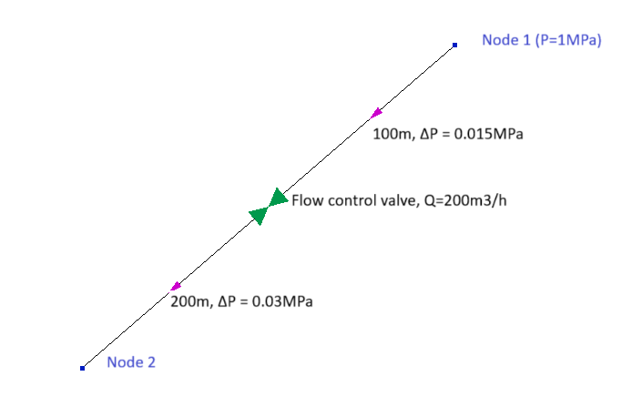
This figure shows an example of a pipeline in which the fluid is pumped from node 1 (with a pressure of 1 MPa) to node 2; the flow rate is maintained at 200 m3/h using a flow control valve. The pressure losses in the pipes before and after the control valve at this flow rate are 0.015 and 0.03 MPa, respectively. Thus, as can be seen, in node 2 of this pipeline the pressure can be practically any value below 0.955 MPa (1 - 0.015 - 0.03 MPa). For example, if the pressure in node 2 is 0.5 MPa, this means that the pressure drop on the flow control valve should be 1 - 0.5 - 0.015 - 0.03 = 0.455 MPa. And if the pressure in the 2nd node is, for example, 0.7 MPa, then the pressure drop across the valve should be 1 - 0.7 - 0.015 - 0.03 = 0.255 MPa, etc. That is, the control valve can maintain the required flow rate at any pressure difference at the system boundaries (only within reasonable limits - see the next paragraph for more on this). But depending on this difference, the valve adjustment parameters (the valve pressure drop and set Kv coefficient value) will be different. Therefore, to determine them, it is necessary to know the pressure at some point in the system both before and after the valve.
Please note that in the Hydrosystem you can also model the operation of the control valve in a mode that is impossible for it, namely, so that a negative pressure drop occurs on it. For example, this can occur if the pressure in node 2 is set for the pipeline in the figure above, for example, 1.5 MPa. As you can easily see, the pressure drop on the control valve in this case will be 1 - 1.5 - 0.015 - 0.03 = -0.545 MPa. That is, the valve should not create additional resistance, but on the contrary - increase the pressure of the pumped fluid by the corresponding value. Of course, a real control valve is not capable of this (the valve can only reduce the pressure), but such a situation is allowed in the calculation - in this case the program will show a corresponding message in the calculation log (about the negative pressure drop on the valve), but the calculation will not be interrupted. This option is convenient to use in cases where it is necessary to calculate what additional pressure should be given to the pumped fluid to provide the required flow rate for it (for example, when calculating the required pump head). So if, as a result of calculating a pipeline with a control valve, it turns out that the pressure loss on the valve is negative, this means that in order to maintain the specified flow rate of the fluid, it is necessary to install not a control valve ("squeezing" the flow in the pipeline), but an additional booster pump with a pressure difference equal to the modulus of the pressure difference calculated for the control valve.
Boundary conditions for waterhammer calculation
The boundary conditions for calculating waterhammer is described in detail in the corresponding section.
________________________________________________
* - this pipeline model is considered just as an example. All the above reasoning and conclusions will be valid for pipelines with absolutely any topology (branched, unbranched, with one or several start/end points, with closed loops and without, etc.), which everyone can easily verify by compiling this system of equations for any pipeline of interest.
** - if there are inflows/outflows in intermediate nodes, nothing will change in principle in the system of equations for this pipeline. Only in the right part of each of the last four equations there will be not zero, but the value of the inflow/outflow in the corresponding node, which in this case is specified in the input data and is a known value in the calculation.
*** - an attentive reader may object at this point that this system may still have a solution if the flow rate QA can be determined by the flow rate balance equation at node 3, for example, if the flow rates QB and QC are specified, or can be determined indirectly by the flow rates in the remaining pipeline branches. However, this means that the user in this case can easily calculate the flow rate QA by himself and specify it in the initial data in the program. Therefore, in order to avoid unnecessary complication of the program's calculation algorithm, only such calculation tasks formulations are allowed in which either the pressure or flow rate value is specified for each initial and final point of the pipeline.