Additional parameters for waterhammer calculation
Waterhammer is a transient process in a pipeline system - i.e., the process of transition of the operating mode of a given system from one stationary state to another. For example, the calculation of waterhammer caused by the closing of a valve is the calculation of the process of transition of a pipeline from the state in which the valve is open to the state in which it is closed. Therefore, to perform the calculation of waterhammer, first of all, it is necessary to calculate the stationary (steady-state) flow (isothermal flow analysis, diameters calculation or thermal calculation), the results of which will serve as the starting point for modeling the waterhammer transient process.
In addition, to perform the calculation of waterhammer, it is also necessary to specify a number of additional parameters and settings. For convenience, the tabs and fields with these parameters are highlighted in a separate color (green) in the program windows. These include:
Like all other transient processes, the waterhammer process is initiated by various types of events. Hydrosystem provides a calculation of waterhammer caused by the following types of events:
valves closing (gate valves, butterfly valves, etc.)
valves opening (gate valves, butterfly valves, etc.)
pumps start up
pumps trip
It is possible to specify one or several different (including non-simultaneous) events. To specify such event, select the corresponding piping component causing waterhammer (valve or pump) and open the "Waterhammer" tab for it in the Object Properties Window.
For valves on this tab, you need to set the following parameters:
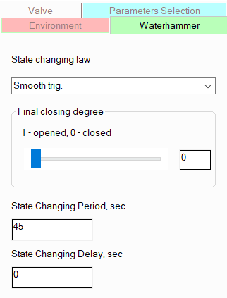
state changing (opening or closing) law - this parameter is used to describe the character of change of the valve capacity in time. That is, in essence, it is necessary to specify here the type of dependence of the fluid flow through the valve on the position of its locking element (rod, shutter etc.). For different types of valves, this dependence can have different forms - it can be close to a linear function and various smooth dependencies (to a polynomial spline or a cosine trigonometric function). The nature of this function for the valve in question can usually be found either in reference literature or in its passport data. However, it should be remembered that at a smooth change in the state of the valve, the waterhammer pressure rise depends quite weakly on the form of this function (it depends much more on the opening/closing speed, and even then not in all cases). Therefore, even if you select an incorrect function (for example, in the absence of data on the valve), the calculation error will not be dramatic. Also, for the valve, you can specify an abrupt (momentary) change in state, which will be considered as opening/closing of the valve in an infinitely small period of time. By default, the persistent state is selected for the valve;
final closing degree of valve - here you can specify the final position of the valve's locking element, thus simulating its partial opening and closing. However, in the current version of the program, this calculation is only available in beta testing mode and only for "end" valves (which are the last elements in the branch);
state change period - the duration of the valve opening/closing is indicated here;
state change delay - here you need to specify the moment in time at which this event (valve closing/opening ) starts to occur. If we a waterhammer process caused by a single event (or several simultaneous events) is considered, then specifying a state change start time N different from 0 does not make sense. In this case, nothing will happen for the first N seconds, the flow parameters will be constant, so this will only increase the calculation execution time. If it is necessary to calculate a waterhammer process initiated by several non-simultaneous events, then using this parameter you can delay these events in time, specifying for each of them the moment in time (relative to a certain initial reference point - the zero moment in time), at which this event begins to occur. The start time of the first event is usually taken as the initial reference point.
When calculating the waterhammer caused by pump trip/startup, it is necessary to set the following parameters for the pump on the "Waterhammer" tab :
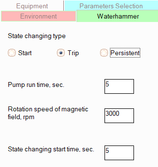
state changing type - by default, the pump is set to a persistent state, but here, if necessary, you can simulate its start or stop (trip);
pump run time - this parameter is determined as follows:
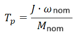
where  is
the total moment of inertia of all rotating masses on the shaft of the
"pump + electric motor" unit (kg*m2) ;
is
the total moment of inertia of all rotating masses on the shaft of the
"pump + electric motor" unit (kg*m2) ;  is the nominal rotation frequency of the electric motor
magnetic field (sec-1);
is the nominal rotation frequency of the electric motor
magnetic field (sec-1);  is the torque of the pump at this frequency (N*m).
The run-out time is an integral parameter characterizing the inertial properties of the rotating parts of the "pump + electric motor" unit. If all the above parameters are available in the pump's passport characteristics (or they can be determined empirically), the run-out time can be calculated directly using the formula above and entered in the corresponding field. If some of this data is difficult to obtain or their reliability is questionable, it is recommended to use some "characteristic" values of the pump run time in the calculation. Practice shows that often an increase in the run-out time even several times does not cause significant changes in the overall picture of the waterhammer process. Therefore, even an approximate value of the pump run-out time can provide acceptable accuracy of the waterhammer calculation;
rotation speed of magnetic field - for "standard" pump impeller rotation frequencies (which in turn are specified in the pump characteristics), this parameter is calculated by the program automatically and does not need to be specified. However, for some frequencies (for example, 1950 or 2650 rpm), this recalculation may not work, so in these cases, you must manually specify the magnetic field rotation frequency;
state changing start time - here you need to specify the moment in time at which this event (valve closing/opening ) starts to occur. If we a waterhammer process caused by a single event (or several simultaneous events) is considered, then specifying a state change start time N different from 0 does not make sense. In this case, nothing will happen for the first N seconds, the flow parameters will be constant, so this will only increase the calculation execution time. If it is necessary to calculate a waterhammer process initiated by several non-simultaneous events, then using this parameter you can delay these events in time, specifying for each of them the moment in time (relative to a certain initial reference point - the zero moment in time), at which this event begins to occur. The start time of the first event is usually taken as the initial reference point.
Boundary conditions at pipeline nodes
For most pipeline nodes, the boundary conditions for waterhammer calculation are predetermined by the calculation method. For example, in branch connection nodes, the boundary conditions are the balance of flow rates in the node and the coincidence of pressures (the pressure values themselves are either specified in the initial data or determined during the calculation of steady-state flow). And the end nodes of the pipeline, which contain "point" hydraulic resistance (for example, the pipe entrance/exit or valves), are considered as nodes of shock wave reflection, and the boundary condition for these nodes is the constant pressure in the node (the value of which, again, is either specified in the input data for the nodes or determined during isothermal, heat or other calculation of steady-state flow). It is not necessary to specify boundary conditions for such nodes.
However, for pipeline end nodes that do not have "point" hydraulic resistances, you can specify different boundary conditions for the calculation. To do this, select such a node and open the "Waterhammer" tab in the Object Properties Window (if this tab is missing for the node, then either this node is not a terminal node or there is a point resistance adjacent to it):
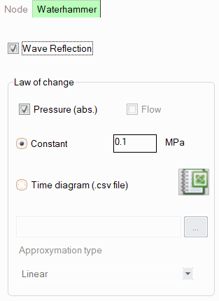
By default, for such a node, the reflection of shock waves is taken into account and the boundary condition is the constant pressure in the node, but if necessary, here it is possible:
enable/disable wave reflection - disabling wave reflection may be required, for example, to model the connection point of the calculated pipeline fragment to another extended pipeline segment that does not need to be calculated (i.e., the shock wave at this node "leaves the pipeline and does not return"). However, it should be understood that this is largely an idealization, since even in a very long pipeline, the shock wave will sooner or later reach its beginning/end (the point of connection of the pipeline with the "outside world") and be reflected back. Therefore, in order for the calculated pipeline model to adequately describe the behavior of a real pipeline system at waterhammer transient event, it is recommended to model a pipeline in its entirety - from the beginning points of the real piping system (where the pipeline is connected to the equipment/devices from which the fluid is pumped) to the end points of the pipeline (where it is connected to the equipment/devices to which this product is fed). Wave reflection should be enabled for such beginning/end points;
boundary conditions (law of pressure or flow change) - are set only if wave reflection is selected. The following can be set as boundary conditions in a node:
the condition of constant pressure is the most common case in practice, since often in the pipeline modeled for calculating waterhammer, the initial/final elements of the piping model are vessels/devices with the pumped fluid, the pressure in which can be considered constant without noticeable error (their minor fluctuations have practically no effect on the picture of the waterhammer process) and independent of the phenomena that occur in the pipeline system;
the condition of constant flow rate - this case is extremely rare in practice, since during transient processes caused by opening/closing valves or switching on/off pumps, the flow rate can remain constant only in very rare "exotic" cases (for example, if the consumer has a flow control device installed that responds very quickly to changes in the flow parameters in the pipeline and continues to maintain a specified constant flow rate even with significant changes in the operating mode of the pipeline system);
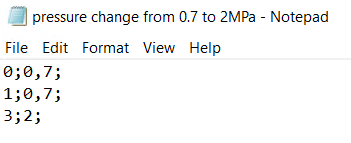
law of flow or pressure change over time - this type of boundary conditions is used if there is equipment/device in a given pipeline node, the pressure/flow in which changes over time due to some "external" reasons (usually related to the process technology in this equipment), not related to the phenomena occurring in the pipeline system itself. These boundary conditions in the node are specified in the form of loading a special .csv file into the program with a table of values, in which the first column is time (in seconds), the second is the parameter (flow or pressure in the units of measurement that are selected for the current project), the separator is a semicolon. As an example, the contents of the .csv file (opened in the standard Notepad application) are given below, using which the following condition is modeled: in the first one second of the transient process, the pressure in the node is constant and equal to 0.7 MPa, in the next two seconds the pressure increases to 2 MPa, after which it remains constant until the end of the transient process:
After loading the .csv file, you must specify the type of approximation of the dependence given in this file (linear, trigonometric or spline) in the corresponding drop-down list. The loaded .csv file can be opened in Microsoft Excel (if it is installed on this computer) by clicking on the corresponding button to the right of the switch.
When setting boundary conditions at the end nodes of a pipeline, you should carefully study the operating principle of the pipeline system and understand what exactly each of the start and end points of the pipeline model is (what they model, the connection of the pipeline to some equipment or something else), and then set a suitable condition for each of them (except for those in which the point element is located).
The calculation results of any transient
process, including the waterhammer process, are most conveniently presented
in the form of graphs of the change in time of the flow parameters in
the pipeline (pressures, fluid velocities, etc.) at the points of interest
in the pipeline. To add such points (in the Hydrosystem they are called
"viewpoints"), you must activate the "Point Values"
command  of the Waterhammer
toolbar, then right-click on the desired location for adding the point
on the pipeline diagram (in the current version of the program, points
can only be added to straight pipes) and select the appropriate item from
the pop-up menu:
of the Waterhammer
toolbar, then right-click on the desired location for adding the point
on the pipeline diagram (in the current version of the program, points
can only be added to straight pipes) and select the appropriate item from
the pop-up menu:

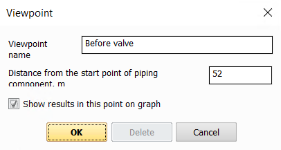
In the window that appears, you need to specify the name of the point and indicate its location relative to the beginning of the selected pipe:
The added point will be displayed
on the pipeline diagram. In the same way, you can edit the name/location
of the already added viewpoint (as well as delete it) by right-clicking
on it on the diagram with the activated "Point Values" command of the Waterhammer
toolbar.
The number of viewpoints for a pipeline is unlimited, but adding a viewpoint "every 10 meters of pipe" usually does not make much sense, since when passing such short distances, the shock wave, as a rule, does not undergo significant changes (neither weakens nor strengthens). Therefore, the calculation results for such points will be identical. Usually, viewpoints are added in the places of the pipeline that are of greatest interest (for example, before and after the valves or pump with a changing state, where, as a rule, the pressure rise has a maximum), as well as in the most "old" sections of the pipeline and elements that can withstand the least load.
Parameters for calculating the shock wave velocity
The magnitude of the pressure increase during a waterhammer, as well as the time periods of oscillations in the flow parameters in the pipeline, largely depend on the speed of propagation of the shock wave. When the program determines the speed of the shock wave, the calculation takes into account both the value of the isothermal speed of sound in the liquid and the correction for the elasticity of thin-walled pipes (the latter only in the case when the outer diameter of the pipeline and the coefficient of elasticity of the pipe wall material are specified).
The isothermal speed of sound in the fluid generally is calculated automatically. However, it is important to note that the thermodynamic library "Properties" does not allow calculating the speed of sound in a liquid, as well as the default thermodynamic model of the Simulis Thermodynamics library. In addition, when manually specifying the thermophysical properties of the fluid, the speed of sound can only be calculated if the compressibility coefficient of the liquid is specified (it is specified among the waterhammer calculation settings on the "Waterhammer" tab of the Object Properties window for the pipeline). Therefore, to correctly take into account the speed of sound when calculating the waterhammer, it is recommended to use the following methods for defining the fluid:
for water - WaterSteamPro library (Water-steam by IAPWS-IF97 equations);
for liquefied hydrocarbons and natural gases - the GERG-2008 library;
for other fluids:
STARS library ,
Simulis Thermodynamics with the LKP thermodynamic model (which adequately calculates the speed of sound in a liquid),
manual input of properties with specifying the coefficient of isothermal isentropic compressibility.
In all other cases, the speed of sound in the calculation will be assumed to be equal to some average value of 1000 m/s.
In addition, to correctly account for the correction for the elasticity of thin-walled pipes when calculating the shock wave velocity, you should specify the outer diameter of the pipeline along with the internal diameter when specifying branches, reducers and other elements with a change in diameter, and also specify the material of the pipeline wall or enter the value of its elastic modulus (coefficient of elasticity). To do this, select the pipeline in the project tree and then open the "Environment" tab in the Object Properties Window:
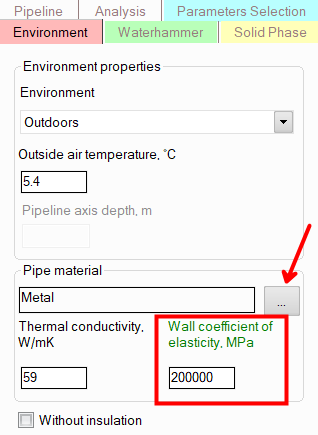
This is especially important for thin-walled pipes of large diameter, since for them the correction for the elasticity of the pipes can be significant.
Waterhammer calculation settings
To set general settings for calculating waterhammer, select a pipeline in the project tree and open the "Waterhammer" tab of the Object Properties Window for it. The following information is displayed there:
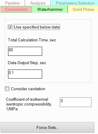
total calculation time shows what period of time from the moment of the onset of the transient process (waterhammer) needs to be calculated. For the calculation, you can select different total calculation times depending on the calculated scenario of the occurrence of a waterhammer and the purpose of your calculation. Do not forget that if a sufficiently long calculation time is selected and the waterhammer calculation takes a long time, it is not necessary to wait for the calculation to complete. The waterhammer calculation can be "paused" at any time using the corresponding button on the Waterhammer toolbar and the calculation results for the time period already calculated at that moment can be displayed. After that, you can continue the calculation or stop it if the required calculation purpose has already been achieved;
data output step - this parameter determines the accuracy with which the calculation results will be displayed on the graphs. The smaller the step, the more accurate the calculation results will be, but the longer the waterhammer calculation will take. And vice versa - the larger the step, the faster the calculation will be performed, but the lower its accuracy will be. Selecting an appropriate data output step for calculating waterhammer for a particular pipeline system is a largely "creative" process. The fact is that the value of the data output step, sufficient to obtain the required calculation accuracy, largely depends on the pipeline structure (on the lengths of the shortest pipe in the pipeline model), on the nature of the events causing waterhammer (sharp/smooth), on the speed of shock wave propagation and many other factors. Therefore, unfortunately, it is impossible to give universal recommendations regarding which data output step should be used in calculations. Usually, in practice, selecting a data output step, is made as follows: first, a waterhammer calculation is performed for a pipeline with a fairly large output step value (couple of seconds, for instance), after which calculations are repeated for smaller steps, gradually reducing the step and comparing the calculation results with the previous ones. As the output step decreases, the calculation results will be more and more accurate (the graphs of pressure fluctuations and other flow parameters will look more and more "physical"), and at a certain value of the output step, there will come a point when the next decrease in the step will not lead to a change in the calculation results that is critical from the point of view of the calculation purpose. In this case, it is considered that the maximum calculation accuracy for a given pipeline model has been achieved and the current output step is optimal for it. Further decrease in the step in this case does not make sense - it will only lead to a slowdown in the calculation, but will not bring a significant increase in accuracy.
Please note that it is necessary to distinguish between such concepts as the waterhammer "calculation step" of the "data output step" for the results of its calculation. If the output step shows the accuracy with which the calculation results should be output, then the calculation step shows the accuracy with which the calculation itself is performed, and the values of these two parameters may not coincide. The output step is specified by the user in the waterhammer calculation settings, while the calculation step is selected by the program automatically as the smaller of two values - the ratio of the length of the shortest pipe in the pipeline to the shock wave propagation speed and the data output step specified by the user. That is, even if the user has specified a relatively high value of the output step, then in this case the waterhammer calculation will be performed with sufficient accuracy so that the shock wave is "caught" in each, even the smallest, section at least once (it's just that not all of the time points for which the flow parameters were determined will be output in the calculation results). And if the user specifies a small value of the output step, then the calculation step is taken the same in order to guarantee the specified accuracy of the results.
use specified below data - if this option is disabled, the following settings will be used to calculate the waterhammer:
the data output step will be taken equal to the step of waterhammer calculation, which, as was said above, is defined as the ratio of the length of the shortest pipe in the pipeline to the speed of shock wave propagation. Such an algorithm for selecting the value of the step allows to obtain good calculation accuracy (thus, the shock wave will be "caught" in each, even the smallest, section at least once) at a relatively high calculation speed. However, in some cases, especially when calculating complex and extended pipelines, the calculation with such a step can take quite a long time. Therefore, to speed it up, the data output step should be increased. The calculation step in this case will not change, but due to the fact that the number of points for which the calculation results will be output will decrease, this will allow to achieve an increase in the overall calculation speed (however, this may lead to less accuracy of the graphs with the calculation results). In addition, if it is necessary to increase the calculation accuracy, the data output step can be reduced - the calculation step in this case will also decrease;
the total calculation time is taken to be equal to the time it takes for the shock wave to pass between the two most distant points of the pipeline, if the waterhammer is caused by an instantaneous event, or, if the waterhammer is caused by a smooth event, to the duration of this event. Calculation with these settings will only calculate the first peak of flow parameter oscillations in the pipeline, so to evaluate the dynamics of flow parameter oscillations (to determine oscillation periods, oscillation damping dynamics, etc.), it is recommended to enable the "Use specified below data" option and set the total calculation time and data output step manually.
consider cavitation - if this option is disabled, the calculation of waterhammer is performed using a simplified model, considering the pumped liquid as a certain idealized fluid that can withstand any vacuum and remains in a liquid state (i.e., no cavitation occurs). Please note that in this case the calculation results may showing the pressure at the waterhammer process drop below absolute zero (which is, of course, not possible) due to simplifications made in this model. Despite the simplified nature of this model, it is excellent for calculating waterhammer, in which the fluid pressure remains at a relatively high level. If the pressure during waterhammer drops below the saturated vapor pressure of the pumped liquid (this can happen, for example, at points in the pipeline after the closing valve or at other points in the pipeline at the moment when a wave of pressure decrease follows the shock wave), then for a more correct accounting of such phenomena, this option should be enabled. In this case, the calculation will be performed taking into account the boiling of the liquid (cavitation), during which the program will determine the places of formation of cavitation caverns, take into account their occurrence and collapse, and also take into account distributed cavitation, etc. However, the calculation itself in this case will be performed a little slower than the calculation without taking into account cavitation, which can be critical for complex and extended pipeline systems. Therefore, if necessary, cavitation accounting can be enabled/disabled.
coefficient of isothermal isentropic compressibility of the liquid (1/MPa) - is set at manual input of the fluid properties for a more accurate calculation of the shock wave velocity.
Calculation and export of the unbalanced forces caused by waterhammer
In addition to calculating the flow parameters in the pipeline (pressures, fluid velocities, etc.), when calculating water ammer, you can also determine the unbalanced forces that arise during a waterhammer between any pairs of viewpoints in pipeline. To calculate such forces, first of all, you need to specify between which pipeline viewpoints (for more information on specifying viewpoints, see above) they need to be determined. To do this, select the pipeline in the project tree, open the "Waterhammer" tab of the Object Properties Window for it and click the "Force sets…" button in it:
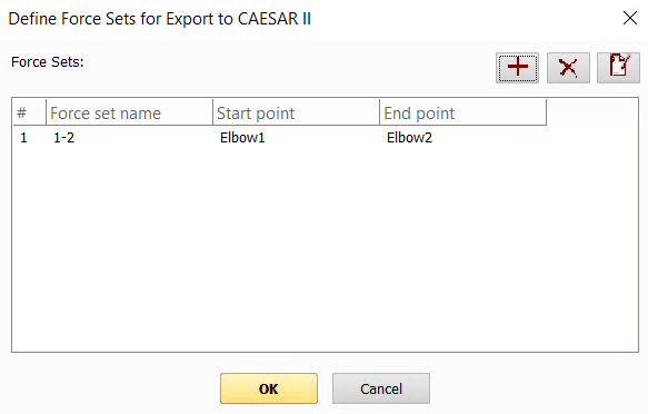
To add/remove/edit forces tables in the window that appears, use the corresponding buttons in the upper right part of this window.
When specifying tables of forces for points between which the force will be calculated, you can enable or disable the incorporation of forces at the point itself. Disabling the incorporation the value of force at a point may be required in cases where this point is on the boundary of the pipeline calculation model (for example, in a plug, equipment, junction with another pipeline, etc.) and if there is confidence that this part is fixed good enough to perceive forces and do not transfer them to the part of the pipeline under consideration (for example, there is an anchor in this point or an equipment support). Otherwise, the forces at the point should be taken into account.
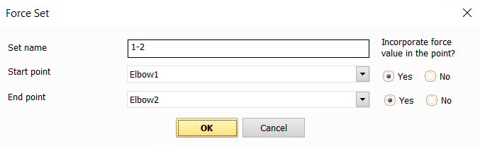
Please note that both viewpoints between which the forces are calculated must be located in the same branch of the pipeline and on the same line.
If force sets are specified for a pipeline, then when performing a waterhammer calculation, in addition to the flow parameter values in the pipeline (pressures, fluid velocities, etc.), unbalanced forces between specified points and their change over time will also be calculated. The calculated forces can then be viewed as graphs of their change over time using the corresponding menu command "Analysis – Charts at Viewpoints" or the Waterhammer toolbar, and also exported to the CAESAR II pipeline stress analysis program (for more information, see here) to take them into account in the piping stress calculation.
The Hydrosystem also provides for the calculation of forces arising at a waterhammer in the nodes and resistances of the pipeline and their subsequent export to the "START-Prof" piping stress analysis software. A detailed description of this function is given here.