Tips and tricks

This section provides a list of practical tasks that are often encountered when working with the Hydrosystem, with instructions on how to solve them and links to the relevant sections of the help system, which describe them in detail.

How to model rectangular/square cross-section of pipeline, 'pipe in pipe', etc.

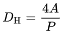
In the calculations in Hydrosystem only round pipes are considered, however pipes and channels of any other shape can also be modeled in the program as a regular cylindrical pipe with a diameter equivalent to a given non-circular section. In hydrodynamics such a diameter is called "hydraulic diameter" (or "equivalent diameter"). It is defined as:

where DH is the hydraulic diameter, A is the cross-sectional area of the pipe/channel, P is the wetted perimeter of the cross-section (with which the pumped fluid is in direct contact).

Research shows that when using the hydraulic diameter, the turbulent flow friction losses equations obtained for round cross-section pipes remain valid for pipes and channels with other shapes. Below are the formulas for calculating the hydraulic diameter for some common cross-section shapes:

How to model a cap/plug

There is no special "cap" element in the Hydrosystem, but it can easily be modeled as a closed valve (of any type). How to model a closed valve is described in detail here.

How to model non-standard pipeline elements

There are several ways to model any elements of the piping system that are not included among the standard element types in the Hydrosystem:

1. As a component with known loss coefficient. The local loss coefficient for an element can be found in the relevant reference literature (for example, in reference databooks on hydraulic resistance by Idelchik, Miller, Crane and other authors) or in the passport characteristics of the modeled component/device. If the local loss coefficient is unknown, but the pressure drop on an element is known (for a certain fluid with a certain flow rate/speed) or there is a dependence of the pressure drop on the flow rate, then the local loss coefficient can be easily determined through the pressure drop using the well-known Weisbach equation (Δp=ζ*ρw2/2, where ρ and w are, respectively, the density and velocity of the fluid, Δp is the pressure drop, ζ is the local loss coefficient). Please note that the Weisbach equation shows the relationship only between the local hydraulic resistance of the element and the flow velocity and properties. Therefore, if a hydrostatic pressure drop also occurs on the modeled element (if the points of flow entry and exit from it are at different heights), it is necessary to clarify whether the known pressure drop on the element includes this hydrostatic component or not. If it does, then it must be subtracted from the pressure drop and modeled separately (as an elevation change element), and the local losses coefficient must be calculated using the Weisbach equation based on the remaining "local" part of the resistance. If the known pressure drop on an element represents only local losses on that element, then the local loss coefficient must be calculated based on this value (without subtracting anything from it), but the hydrostatic losses must still be modeled separately as the corresponding elevation change;

2. As a valve with a known flow coefficient Kv. This method is suitable mainly for valves of various types, for which the value of the flow coefficient Kv (or Cv, for which the Kv can be calculated as Kv = 0.864*Cv) can be found in reference literature, in the passport characteristics or in the manufacturer's catalog;

3. As a component with known change of pressure and/or temperature (if this drop is known explicitly for this element). This element should be used with caution, since it will adequately describe the behavior of the piping element being modeled only in the case when the fluid flow rate through this element is a known and constant value. If the flow rate through this element is unknown/not fixed, a component with known change of pressure and/or temperature should not be used (for more information, see here).

How to model various equipment

When modeling equipment, it is important to distinguish between "flow-through" devices, where the flow remains continuous, and devices in which the flow brakes. Heat exchangers of various types can be used as an example of the first type of devices, and a tank in which the flow enters above the liquid level and is discharged, of course, below it can be used as an example of the second type. Modeling devices with a flow break is described in detail here. As for flow-through devices, they can be modeled in several ways:

1. As a component with known change of pressure and/or temperature. The pressure drop on the device can usually be found in its data sheet. However, this type of celement should be used with caution, since it will adequately describe the behavior of the piping element being modeled only in the case when the fluid flow rate through this element is a known and constant value. If the flow rate through this element is unknown/not fixed, a component with known change of pressure and/or temperature should not be used (for more information, see here);

2. As a component with known loss coefficient. This method of modeling equipment has no disadvantages of the previous one and can be used in any cases. The total coefficient of local resistance of all elements of the modeled equipment through which the flow passes is not always available in the passport characteristics of the equipment (for some "standard" equipment, such as heat exchangers, these coefficients can be found in reference literature). Therefore, if the local loss coefficient is unknown, but the pressure drop on the device is known (for a certain fluid with a certain flow rate/speed) or there is a dependence of the pressure drop on the flow rate, then the local loss coefficient can be easily determined through the pressure drop using the well-known Weisbach equation (Δp=ζ*ρw2/2, where ρ and w are, respectively, the density and velocity of the fluid, Δp is the pressure drop, ζ is the local loss coefficient). Please note that the Weisbach equation shows the relationship only between the local hydraulic resistance of the element and the flow velocity and properties. Therefore, if a hydrostatic pressure drop also occurs on the modeled equipment (if the points of flow entry and exit from it are at different heights), it is necessary to clarify whether this "passport" pressure drop on the equipment includes this hydrostatic component or not. If it does, then it must be subtracted from the pressure drop and modeled separately (as an elevation change element), and the local losses coefficient must be calculated using the Weisbach equation based on the remaining "local" part of the resistance. If the "passport" pressure drop of the equipment is only a combination of local losses and friction losses, then the local loss coefficient must be calculated based on this value (without subtracting anything from it), but the hydrostatic losses must still be modeled separately as the corresponding elevation change.

How to model inclined pipes

The slope of the pipe (up or down) determines the hydrostatic pressure losses on pipe, so taking it into account is especially important when calculating the flows with high densities - liquids, gas-liquid mixtures and mixtures of liquids with solid particles, as well as "dense" gases (for example, high-pressure water vapor, supercritical fluids, etc.). In the Hydrosystem, the slope of the pipe can be modeled in two ways:

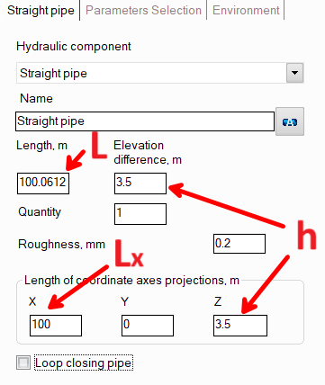
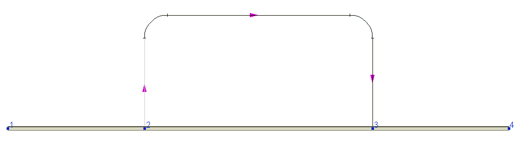
1. Using the projection of the pipe length onto the Z coordinate axis (for more information on modeling pipes, see here). This method is the most accurate, so it is especially recommended for use in calculating flows in which the density of the fluid changes significantly during the flow. In this case, for each section of the pipe, it is necessary to specify the lengths of its projections onto the corresponding coordinate axes in the input data. As an example, the figure below shows a section of the pipe directed along the X axis with an upward slope along the vertical Z axis:

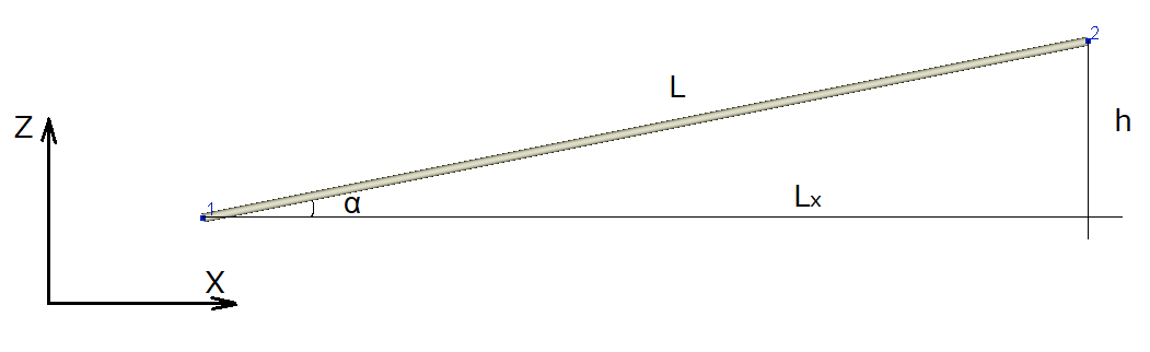
Accordingly, if the projections of this section are known initially, it is necessary to set the length "Lx" (positive value) for it along the X axis, and the elevation difference "h" (positive value, since the pipe 'is directed upwards) along the Z axis.

If the projections are unknown, and only the total length of the pipe L and the slope angle α are known, then "h" and "Lx" can be easily determined as h=L*sin(α), Lx=L*cos(α).

If the length of the pipe "L" and the elevation difference "h" are known, then in the Hydrosystem you can first set the total length of the pipe and the elevation difference on it - in this case, the direction of the pipe will be chosen arbitrarily along the X or Y axis. However, if necessary, it can then be adjusted.

If the pipe has a downward slope, everything is done similarly, only the projection onto the Z axis (or the elevation difference) is specified with a minus sign.

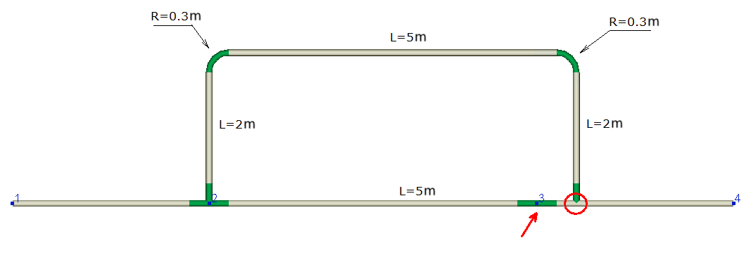
2. Using the elevation change element. An example of using this approach is shown in the figure below:

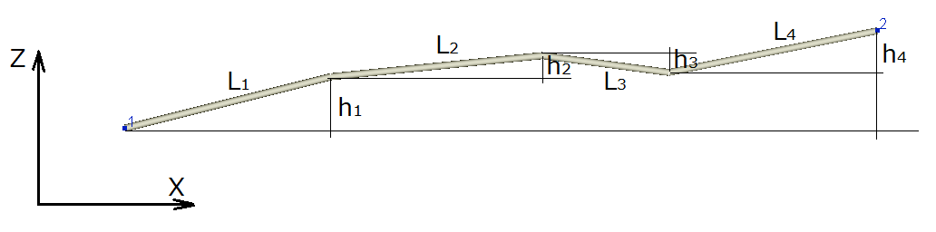
If the piping fragment consists of several sections, each of which has its own length and its own slope value, then in the Hydrosystem such a fragment can be modeled as a sequence of a horizontal straight pipe section with a length equal to L1 + L2 + L3 + L4 and an element "Elevation change" with the elevation difference equal to h1 + h2 + h3 + h4 (note that when adding up, it is necessary to take into account the signs of elevation difference on each of the components - for example, for the pipeline in the figure above, h3 must be with a minus sign, since the 3rd section, unlike the others, goes with a downward slope, not an upward one). That is, friction losses in the pipe are modeled separately as a horizontal pipe, and hydrostatic losses - on the Elevation change element.

This method is more convenient, since you do not have to break the pipeline into separate sections and enter them separately. However, it is less accurate, and it is not recommended to use it when calculating fluids whose densities change significantly along the pipeline. In addition, this method is only suitable for calculating the total pressure drop in pipeline, and using this method it is impossible to accurately calculate the pressure values at any intermediate points of the pipeline (for example, if you need to calculate the pressure at the end of the 2nd section in the figure above, this method will not work).

How to model closed loop pipelines

When modeling pipelines containing various types of closed loops (including bypass lines, fluid recirculation lines, or any other pipeline systems in which the fluid can get from point A to another point B by two or more different paths), it is important to remember that they are essentially modeled the same way as any other types of pipelines. In the same way, a pipeline consists of branches, a branch of piping components (for more information about this, see here), it is just that in this pipeline, different branches will "lead" the fluid by different paths between the same pipeline nodes. Examples of pipeline models of this type are shown below.

1. In the pipeline in the figure below, the fluid is fed from node 1 to node 4 (this fragment is shown in the figure "in volume") and a bypass must be added to it, shown by a thin line:

The initial part of the pipeline consists of three branches: the first branch connects nodes 1 and 2, the second - nodes 2 and 3, and the third - nodes 3 and 4. To model a bypass line, you just need to add another branch to the initial pipeline, directed from node 2 to node 3, and after that, add pipe sections, bends and other elements of this branch. Please note that for the new branch, you need to specify nodes 2 and 3 as the initial and final nodes. If, for example, you direct this branch from node 2 to some other node 5, this will not be treated as a closed loop, but as a flow branch going to a completely different point 5 (even if the positions of nodes 3 and 5 in the piping diagram coincide).

In addition, when modeling pipelines with closed loops, in some cases it is convenient to use the "Loop closing pipe" option for pipes - with its help, you can accurately calculate the dimensions of any section of a closed loop based on the entered lengths of projections of other elements of this loop. The operation of this option can be demonstrated in the example shown above - let's assume that when modeling a bypass line, we made an error somewhere, as a result of which the modeled piping system looks like this:

This error is obvious (in this case it is connected with the fact that the sizes of two elbows were not taken into account), because the piping model in node 3 "diverges". To correct this error, it is necessary to select in the closed loop the pipe section whose projections raises the most questions and turn on the "Loop closing pipe" option for it:

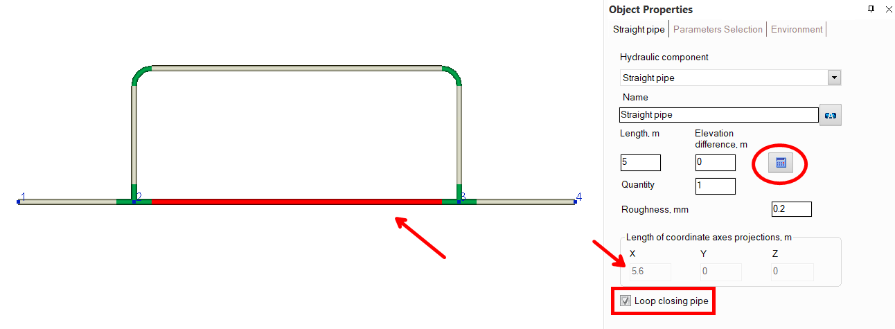
The program will calculate what the projections of this pipe should be so that the loop closes perfectly (this pipe section is shown on the isometric diagram as a pale gray line). In order to then "accept" the lengths of the projections calculated by the program and determine the length and elevation difference on the pipe, click the "Recalc by graphics" button (in the form of a blue "calculator") for this pipe.

Please note that this button is displayed only if the "Scaled graphic view" and "Show all components" options are enabled in the pipeline graphic view options (on the View Options toolbar) and the "Precise graphic representation of scaled view" option is enabled in the program settings. Otherwise, it is not recommended to use the "Loop closing pipe" option, since when the display of piping components and/or scaled view are disabled, the calculation of the projections of the closing pipe may be incorrect. It should also be noted that if the "Recalculate elevations and angles on graphic before every analysis" option is enabled in the program settings, there is no need to click the "Recalc by graphics" button for each closing section. At the calculation, the parameters of all closing pipes in the pipeline will be automatically recalculated according to the projection lengths defined by the program.

The "Loop closing pipe" option is recommended to be used only in cases where you are not sure of the correctness of the entered length/projections of some section of the pipeline. If the closed loop is correctly modeled, there is no need to use this option.

2. The figure below shows a piping system in which the flow is pumped "in a circle" by a pump:

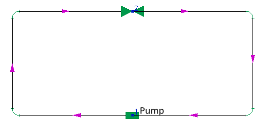
To model such a pipeline in the Hydrosystem, it is necessary to add two branches to the pipeline - one directed from node 1 to node 2, the other - from node 2 to node 1. After that, it is necessary to add all the components (pipes, bends etc.) to these branches. It is important to mention here that formally this pipeline could also be constructed as consisting of a single branch with the same start and end node - for example, like this (directing the branch from node number 1 to node number 1):

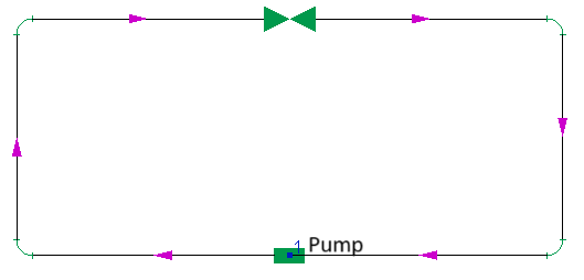
However, unfortunately, at the moment the Hydrosystem does not support calculations of pipelines in which the loops consist of one branch, so it will be impossible to calculate such a pipeline - a closed loop must be made up of two (or more) branches.

3. The figure below shows another example of a closed loop pipeline (including nodes 2, 3, 4, 5, 7):

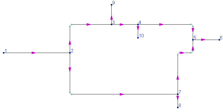
To model this pipeline in the Hydrosystem, the following branches must be added to it:

After that, it is necessary to add all the components (pipes, bends etc.) to these branches. These branches can be added in any order - for example, you can first build a closed loop and then add inlet and outlet branches to it. Or you can first model the flow path from node 1 to node 6 along one of the "routes", then add a parallel path and then add branches going to nodes 8, 9 and 10, etc. The order of the branches is just an order of the equations in the system of equation that will be solved at calculation of these pipeline, which is, of course, not crucial for solving the system of equations. The key thing in modeling such pipelines is that all the branches are added to the pipeline and the correct numbers of the initial and final nodes are specified for all of them.

Please note that during the modeling a closed loop at some point (before it is completely built) the loop may "break", and the same node may end up in two positions. For example, here is how the piping system shown above will look at the moment when the last branch from node 7 to node 5 was added to it (while all other branches were already modeled) and only the first pipe section was added to this branch:

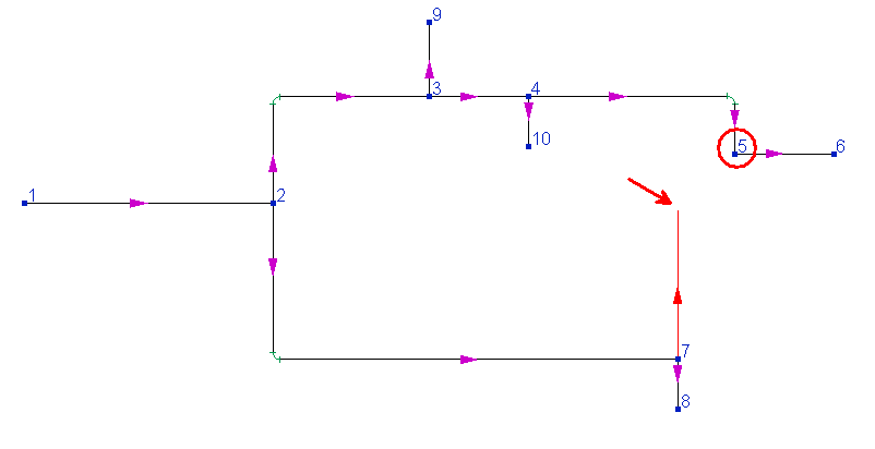
At this point, node 5 will be in two different positions at the same time. This is absolutely normal, since the closed loop modeling is not yet completed. As soon as the last component of the last branch is added, all such "gaps" will be eliminated and each point of the pipeline will be in its place (provided that all elements of the pipeline are modeled correctly, without errors - the occurrence of errors in closed loops is described in detail here).

In addition, when modeling closed-loop pipelines, it is important to remember that an accurate representation of the piping model on the graph can only be achieved by enabling the "Scaled graphic view" and "Show all components" options in the pipeline graphic view options (on the View Options toolbar) and the "Accurate graphic diagram when presented to scale" option in the program settings. Otherwise, the piping diagram will be presented in a simplified form without taking into account the actual sizes of the elements (or even their directions in space) on graphics. For example, here is how the same piping system shown above is displayed when the "Scaled graphic view" is disabled:

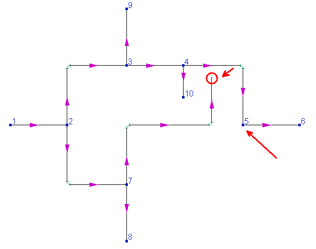
For calculations, this is, of course, not essential, but for ease of working with such piping systems, it is recommended to model them with the "Scaled graphic view" and "Show all components" options enabled.

Also, when modeling branches that make up a closed loop, it should be remembered that the directions of these branches are not of fundamental importance when performing isothermal flow analysis and heat and hydraulic calculations. Even if a branch is modeled in the direction opposite to the flow direction in it, this will not affect the calculation in any way - the flow rates in all intermediate branches of the pipeline are calculated automatically at the pipeline analysis, the program will simply calculate a "negative flow rate" for such a branch (for more information, see here). So it is not necessary to follow the correct directions of branches when modeling closed loops. This is important only when performing pipeline diameters calculation, since for this type of calculation, the specified flow directions will affect what diameter is required for which branch.

How to model control devices

If the control device (flow, pressure or other parameter regulator) has already been sized and its characteristics are known, then it can be modeled as a valve with a known value of the flow coefficient Kv (for more information, see here) or as a component with known change of pressure (if the pressure drop on the control valve is known). If the regulator setting parameters are unknown and need to be determined, then for these purposes you can use the control valve element (if you need to size flow control device) or the parameters selection service (for sizing pressure control devices, flow control devices and other regulators).

How to close pipeline branches

In some cases, it may be necessary to calculate the pipeline operation mode when some of its branches are closed (for example, if some sources and/or consumers are disconnected or some 'bypasses' are closed). In this case, you just need to add any type of valve to such a branch and set it to a closed state. For gate valves, this state is modeled by a relative rod height equal to zero, for butterfly valves - a closure angle of 90 degrees, for all other types of valves - the coefficient Kv=0 (for more details, see here).

How to insert valve or other component in the middle of a pipe

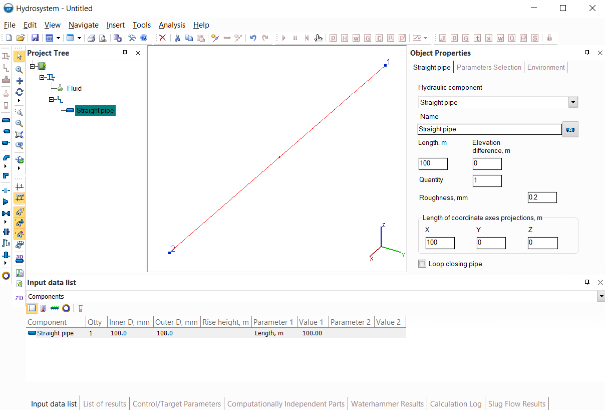
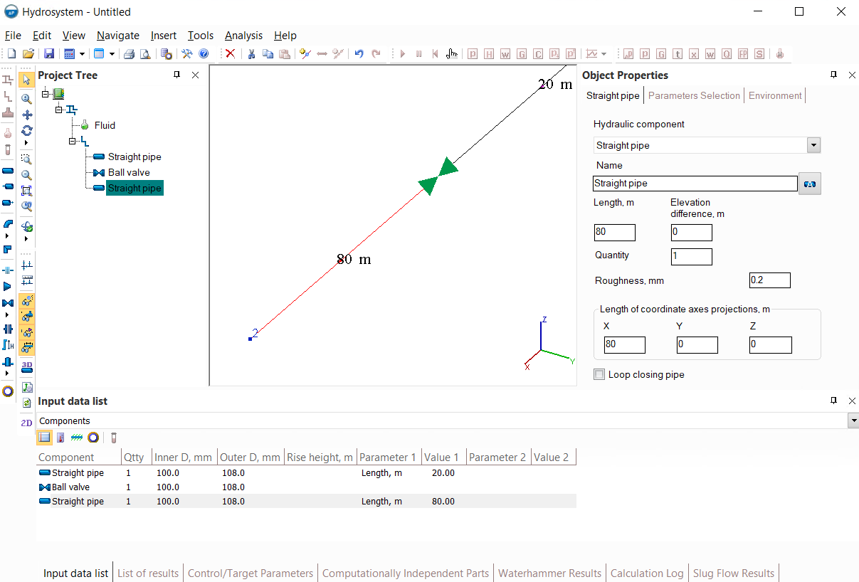
Below is an example of a pipeline consisting of one pipe 100 meters long, into which it is necessary to insert, for example, a ball valve 20 meters from the beginning of the pipe:

There are two ways to do this:

1. Set the length of this pipe to 20 meters instead of 100, add a ball valve after it, and then add another pipe 80 meters long after the valve:

2. Insert a node at a distance of 20 meters from the beginning of the pipe, after which either at the end of the first or at the beginning of the second of the two resulting branches add a ball valve:

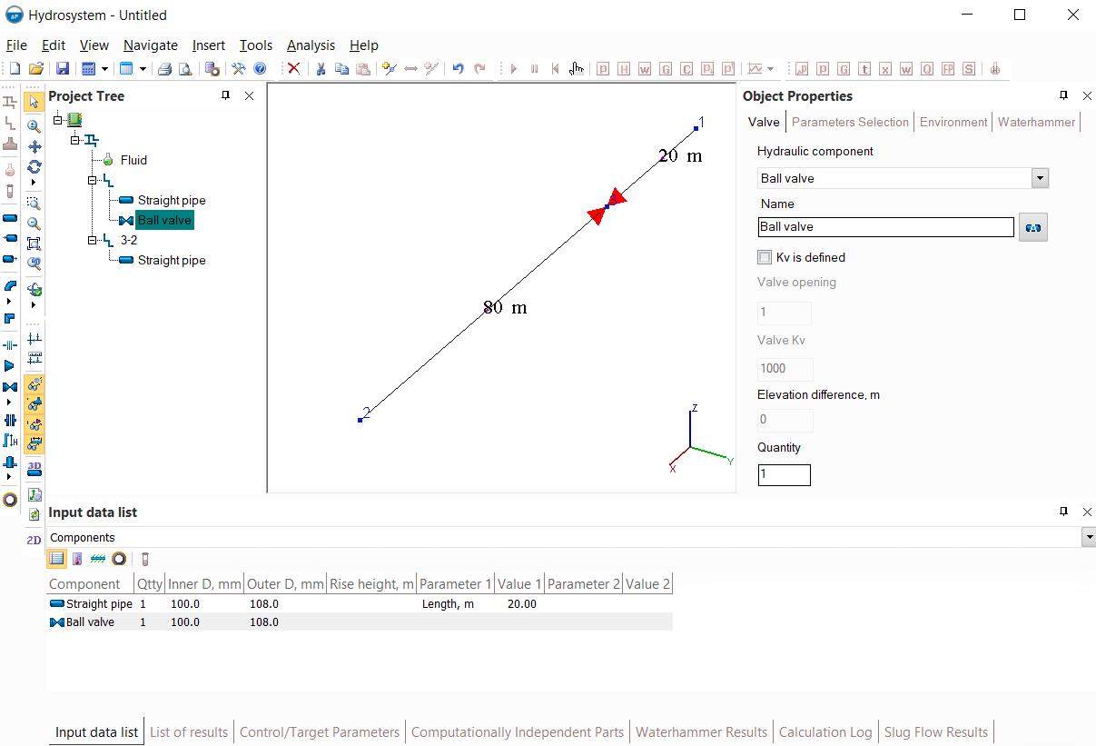
Both methods are equivalent from the calculation point of view, so you can use either of them. However, the first method is more "elegant" since it does not lead to unnecessary division of the original branch into two, which will be more convenient from the point of view of presenting the calculation results. Although, if necessary, in the second method you can then delete the inserted node (for information on how to delete nodes, see here) after you added a valve and get a pipeline model absolutely identical to that obtained by the first method.

How to copy/paste/delete pipeline fragments

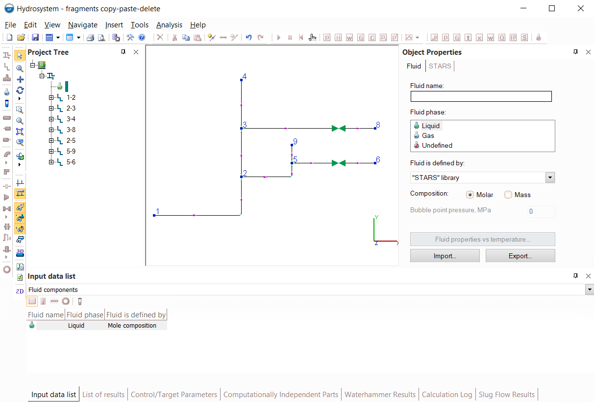
The Hydrosystem provides the ability to copy/paste both separate branches and piping components, multiple branches/components and entire pipeline fragments consisting of several components/branches. Let's consider this using the example of a pipeline shown in the figure below. In this pipeline, it is necessary to copy the fragment from node 3 to node 8 and paste it so that it exits node 4 and goes to a new pipeline node (for example, number 10):

This can be done in several different ways:

Method #1 - copying several elements of a branch. To do this, you need to:

1. Add another branch to the pipeline and set node 4 as its starting point and node 10 as its ending point;

2. Select all components from the "3-8" branch (except the tee) in the graphics window or in the project tree - to select several elements, select the first of them and then, pressing and holding the Shift key, select the last one (if you need to select not all, but only some of the elements of this branch, after selecting the first element, press and hold the Ctrl key and click on all the elements that need to be selected in turn);

3. Select the Copy command of the Edit toolbar or the Edit menu (or simply press Ctrl+C on the keyboard);

4. Select the branch added in step 1 from node 4 to node 10 in the project tree and select the Paste command of the Edit toolbar or the Edit menu (or simply press Ctrl+V on the keyboard).

Method #2 - copying the entire branch. To do this, you need to:

1. Select the original branch "3-8" of the pipeline in the project tree and copy it by selecting the Copy command of the Edit toolbar or the Edit menu (or simply press Ctrl+C on the keyboard);

2. Paste the copied branch by selecting the Paste command of the Edit toolbar or the Edit menu (or simply press Ctrl+V on the keyboard). Note that the pasted branch in the project tree will have the same name as the original one, but the numbers of the start and end nodes will be completely different - not related to the rest of the pipeline. Therefore, the next step is to:

3. Change for the inserted branch its start node to node 4 and its end node to node 10.

Please note that you can also copy/paste multiple branches the same way by selecting several branches in the project tree using Ctrl or Shift keys.

Method #3 - copying a pipeline fragment from one node to another. For more clarity, let's consider this using the example of copying a fragment from node 2 to node 6 and inserting it into node 4 (so that this fragment consists of not one, but two branches). Unlike the case of copying elements between nodes 3 and 8 discussed above, here copying a separate branch or components of a branch will not be entirely convenient, since you need to copy several elements from different branches. Therefore, in this case, it is more convenient to use copying a pipeline fragment from one node to another. To do this, you need to:

1. Select node 2 on the piping diagram, press and hold the Shift key, then select node 6 on the diagram;

2. Select the Copy command of the Edit toolbar or the Edit menu (or simply press Ctrl+C on the keyboard);

3. Select node 4 on the diagram into which you need to paste the copied segment;

4. Select the Paste command of the Edit toolbar or the Edit menu (or simply press Ctrl+V on the keyboard) - the copied branches will be pasted into the project tree under the same names as the original branches, but with appropriate node numbers (the program will assign the first unused numbers to the new nodes) and no further editing will be required.

Each of the methods may be more convenient than others in certain cases, so it is recommended to use them depending on the situation.

Similarly, you can cut or delete fragments of pipelines.

How to swap branches in a project tree

First of all, it is important to remember that the order of branches in the project tree does not matter for the calculation. However, for convenience, it may be necessary to swap some of the branches. To do this, select the branch that needs to be "moved", then cut it to the clipboard (using the Cut ccommand of the Edit toolbar or the Edit menu, or using the Ctrl+X keyboard shortcut), then select the branch after which the cut branch should follow and use the Paste command of the Edit toolbar or the Edit menu (or use the Ctrl+V keyboard shortcut).

You can "move" several branches in a similar way. To select several branches, select the first one, then press and hold the Shift key and select the last one (if you need to select only some of the branches, then after selecting the first branch, press and hold the Ctrl key and click on all the branches you want to select in turn). Then similarly use the Cut and Paste commands for several branches.

How to simultaneously change the parameters of several pipeline elements

The Hydrosystem provides the ability to change the parameters of branches or individual piping components in groups. To do this, they must be selected in the project tree or in other program windows, after which the Object Properties window will display the parameters that can be changed for them simultaneously. For branches, these will be the values of diameters, flow rates, temperatures, roughness and other characteristics, for piping components - location parameters, thermal insulation, etc.

To select several elements (branches or piping components), select the first of them and then, pressing and holding the Shift key, select the last one (if you need to select not all, but only some of the elements, after selecting the first, press and hold the Ctrl key and click on all the elements that need to be selected in turn).

How to model different location, thermal insulation, etc. for different parts of the pipeline

Different location parameters for different pipeline elements can be modeled in two different ways. The first way is to use inheritance of environment, insulation, etc. parameters, as described here. The second way is to use group replacement of these parameters (as described here), selecting those elements for which it is necessary to specify location, insulation, etc. parameters different from the previous ones.

How to automatically calculate elevation differences on elbows and reducers

For this purpose, the Hydrosystem has a separate special function, its operation is described in detail here.

How to calculate diameters only for the part of the pipeline branches (if the diameters for the rest branches are known)

In practice, there are cases when the configuration of a part of a pipeline is already known (for example, this part was designed earlier or even already built and another designed section of the piping system is connected to it), including the diameters of its branches, and it is necessary to select diameters only for the rest of the pipeline. In Hydrosystem, for such cases, you can perform diameters calculation of a pipeline with partially specified diameters. That is, you need to specify them in the input data for those branches for which the diameters are known, and do not specify them for the rest. At the diameters calculation, the program will calculate only the diameters of the branches for which they were not specified, and will leave the specified ones unchanged.

How to calculate the required pump head

The calculation task of the required pump head analysis is usually stated as follows: the initial pressure (P1) at the point from which the pump pumps the fluid is known, the pressure that needs to be obtained at the consumer point where the fluid is supplied (P2) is known, and the flow rate of the fluid that needs to be pumped is known (Q). The required pump head (H) is unknown:

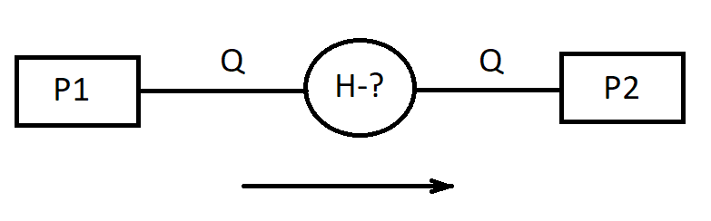
In practice, this calculation task is usually divided into two separate tasks. First, the part of the pipeline before the pump (the suction line) is calculated separately. The initial pressure P1, the required fluid flow rate Q are set as boundary conditions for this calculation, and the final pressure is determined - that is, the pressure at the pump inlet.

Then the pipeline part after the pump (discharge line) is modeled and calculated separately. The final pressure P2, the required fluid flow rate Q are set as boundary conditions for this calculation, and the initial pressure is determined - that is, the required pressure at the pump outlet.

The pump inlet pressure is then subtracted from the calculated pump outlet pressure, and the resulting difference is the pressure difference that must be applied to the fluid so that it is pumped at the required flow rate - that is, the required pump head (in units of pressure, but it can easily be converted to head by dividing it by the density of the liquid and the acceleration due to gravity). If you then want to automatically select a pump based on the calculated parameters, this is described in detail here.

A special case is the calculation of the required pump head for a circulation system, when the pump pumps the fluid in a closed-loop pipeline. However, the principle of solving this calculation task is absolutely the same, it is just that the values of pressures P1 and P2 in this case will be the same. In addition, it is important to remember that since the density of the liquid, and therefore its hydraulic losses, practically do not depend on the absolute value of pressure, for circulation systems it is possible to set any (within reasonable limits) values of pressure as P1 and P2, the main thing is that their values are the same.

The task of calculating the required pump head can also be solved within a single pipeline (without dividing the pipeline model into a separate suction and discharge line), by specifying the entire pipeline and modeling the pump as... a control valve. At first glance, this may seem strange (that the pump is modeled as a control valve), however, as already mentioned here, the pressure drop on the control valve in the calculation results may well be a negative value. This indicates that the pumped fluid must be given additional pressure to provide the required flow rate. And the value of this pressure will be the required pump pressure difference - the program will automatically calculate it and show it in the results as the pressure drop on the control valve.

How to export the calculation results tables without formatting (only data)

To export only the contents of tables with the input data and calculation results (without title blocks and other formatting), when outputting calculation results, select the output to the Microsoft Excel format and specify "Only data from table object(s)" in the output options. More details on this are available here.

Is it allowed to not specify some of the components of the pipeline system?

Of course it is allowed. The designer's task is not to "reproduce" a real pipeline in its calculation model as accurately as possible, but to create an adequate calculation model of this pipeline, which will take into account all the components and parameters important for this calculation. Therefore, if some elements of the piping system can be neglected in the calculation without losing accuracy, then they can be omitted. For example, if you're performing a hydraulic calculation of a 2 km long pipeline, which has one gate valve, then most likely the hydraulic resistance of this valve will be negligible compared to the pressure losses in two-kilometer pipes. Therefore, when modeling this pipeline, the valve can be omitted. However, if you need to calculate the waterhammer caused by the closure of this valve, then it must be modeled. Thus, depending on the context and the formulation of the calculation task, the same element of the pipeline in one case can be very important, in another - not.