Hydraulic calculation of two-phase gas-liquid flow

Two-phase gas-liquid flow can be analyzed ignoring mass transfer between phases (so-called “frozen” flow) or taking into account vaporization and condensation. Frozen flow analysis can be performed both for isothermal flow and as a heat and hydraulic calculation. Calculation taking into account mass transfer between phases (vaporization and condensation) is possible only with combined heat and hydraulic calculation. This calculation requires phase equilibrium calculation, therefore the calculation is possible only when specifying the fluid using the STARS, WaterSteamPro (Water/steam according to IAPWS-IF97), GERG-2008 or Simulis Thermodynamics libraries.

Gas-liquid flow is considered to be steady, and phases are considered to be in the state of thermodynamic equilibrium and having the same temperature and pressure. “Slippage” of liquid and gas phases can be considered; i.e., their movement at different flow velocity. During hydraulic analysis of a two-phase gas-liquid flow, the pattern of two-phase flow at different points along the pipeline is found, and for all components the following values are calculated:

• two-phase flow pattern at various points in the pipeline;

• void fraction (and on its basis, calculation of true phase velocities, as well as hydrostatic losses in components due to elevation change);

• friction losses;

• losses on local resistances;

• losses due to flow acceleration;

• Mach number.

Various methodologies can be used for determining flow pattern and performing the analysis. Since analysis methods for two-phase flows are currently developing and at this point no universally accepted approach exists, Hydrosystem utilizes a number of methodologies for different calculations, from which the user can select the most appropriate methods for any given task. There is also a high degree of flexibility in which methodologies should be used for various types of components in different situations, which can be set using special rules for choosing two-phase calculation methods. User defined rules may be used as well as one of the predefined rules included in the software.

Flow patterns

The two-phase flow pattern is determined using the most popular recently so-called "mechanistic" models based on modeling the physical mechanisms of flow pattern change. A list of implemented methodologies (models) is provided below. The software recognizes and determines 6 flow patterns: stratified smooth, stratified wavy, intermittent, bubble, dispersed-bubble, annular (or annular-mist). At present, the software cannot differentiate variations of these patterns; for example, variations of intermittent pattern (such as slug, elongated bubble and froth) or annular pattern (annular mist, annular wavy or wispy annular). An ability to do this is planned for a future addition.

The calculated flow patterns can be used for a more adequate methodology selection for analyses of void fraction and head loss. An addition of specific analysis methodologies for these variables based on models of various flow patterns is planned in the future.

In addition to determining the two-phase flow pattern, the program also allows to diagnose the possibility of an "severe slugging" two-phase flow occurrence caused by the accumulation of the liquid phase of the fluid before some piping components. Usually, such accumulation takes place at the end of extended horizontal or inclined downstream sections of the pipeline, followed by fluid lifting on vertical pipes. In this case, the accumulation of the liquid phase before lifting can cause a complete overlap of the tube section with liquid, as a result of which the pumping of the gas phase will be carried out by periodic "firing" portions. Such flow regime may cause vibrations of the pipeline and adjacent objects, and also leads to uneven pumping of the gas-liquid mixture. The possibility of occurrence of an severe slugging flow in the Hydrosystem is determined in accordance with the methods described in [32-39].

Void fraction (a.k.a. true volumetric gas content)

To calculate the true volumetric gas content, the program implements a number of correlation types: HEM (homogeneous equilibrium flow model for two-phase flow), power type (Butterworth type) correlations, correlations based on drift flux model and most popular empirical correlations. Currently, power type correlations present more of a historical interest and are utilized for comparison and compatibility with other software. For high and medium flow velocity, the use of Premoli correlation is recommended, while for low flow velocity, Rouhani, Dix-Ghajar-Woldesemayat or Goda-Hibiki-Kim-Ishii-Uhle correlations (depending on slope angle) are recommended. A comparison of applicability and accuracy of various methodologies can be found in [21].

The calculated void fraction is used in the analysis of pressure loss due to elevation change, as well as some other variables (true flow velocity for phases, etc.).

Friction losses

To calculate friction losses of a gas-liquid flow, the program implements two types of correlations: based on homogenous flow model and using two-phase multipliers.

The first group of methodologies calculates loss due to friction as for a single-phase flow with thermophysical properties of a gas-liquid mixture. The two-phase nature of the flow is taken into account in the analysis of the mixture’s viscosity (in the Beattie-Whalley methodology) and the Reynolds number of the mixture (in the Shannak methodology).

The second group of methods calculates loss due to friction for single-phase flow (for gas or liquid phase) with a subsequent correct for multipliers taking into account the gas quality and phase properties. The methodologies of Friedel and MSH are somewhat expanded in Hydrosystem by utilizing the hydraulic friction coefficient from Churchill’s formula (as recommended in [13]) in the analysis, which allows their application for the entire spectrum of Reynolds number, as well as a consideration of the effect of pipe wall roughness. Guidelines for applying the methodologies of two-phase multipliers proposed by Whalley (see [2]) are provided in the table below. More detailed information is provided in [27].

Local losses

The question of analyzing minor head loss (local losses) for gas-liquid flow remains poorly investigated at this time. The current version of Hydrosystem utilizes the main methods of analysis suggested in the literature for this scenario, which are variations on the method of two-phase multipliers for local resistance. Guidelines for applying these methods for various types of local resistance are provided in [13, 30, 31]. For local resistance types where no guidelines are available, the HEM methodology is used.

Acceleration losses

Losses due to acceleration of flow is calculated using the HEM model according to guidelines [1] for adiabatic flow.

Mach number

The Mach number for “frozen” flow is calculated using the model of homogenous frozen flow. An “isothermal” speed of sound is used in gas phase. Mach number for flow with mass transfer is determined using HEM model.

Viscosity of the mixture

Average viscosity of two phase mixture is calculated according to Beattie – Whalley method [23].

Calculation of three-phase gas-liquid-liquid flow

The calculation of the three-phase mixtures of gas and two immiscible liquid phases (for example, oil and water) is currently carried out according to the methods of a two-phase gas-liquid flow. In this case, it is assumed that the two liquid phases form a homogeneous liquid emulsion. The density of such an emulsion is calculated using a uniform model and the viscosity is calculated using the Brinkman - Roscoe formula [40-41] that is derived from the well-known Einstein equation [42] with determination and taking into account the type of emulsion (water-in-oil or oil-in-water). The phase inversion point is determined from the condition of the viscosity values equality (i.e., when the viscosity of a water-in-oil emulsion is equal to that of an oil-in-water emulsion).

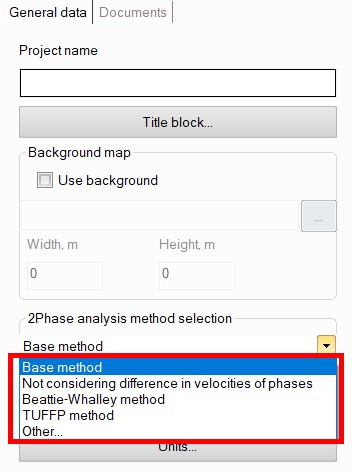
Two-phase flow calculation presets

When installed, the program comes with the following 4 preset profiles with methods for calculating gas-liquid flows, available for selection in the project input data:

The rules for selecting methods of each of the specified profiles are contained in the corresponding XML files in the program installation directory (by default C:\Program Files (x86)\truboprovod\hst_eng):

These include:

• "Base method" (file HST.xml) - this profile contains calculation methods that have the widest scope of application:

• • calculation of the flow pattern using the Barnea method;

  • calculation of the void fraction using the Premoli method;

  • calculation of friction losses using two-phase multiplier methods according to Whalley recommendations:

  • • at low mass flow rate and high values of the ratio of liquid phase viscosity to gas viscosity - the Lockhart-Martinelli method;

    • at high mass flow rate and high values of the ratio of liquid phase viscosity to gas viscosity - the Chisholm method;

    • at low values of the ratio of liquid phase viscosity to gas viscosity - the Friedel method;

  • calculation of local losses according to recommendations [30].

• "Not considering difference in velocities of phases" (file HST_HEM.xml) - the same methods as in the "basic" method, but the homogeneous flow model (HEM) is used to calculate the void fraction.

• "Beattie-Whalley method" (file HST-FR-BW, LOC -HEM.xml) - this profile uses calculation methods that have proven themselves well in the calculation of "transfer" pipelines (pipelines for supplying petroleum in a gas-liquid state from furnaces/heaters to a rectification column):

• • calculation of the flow pattern using the Barnea method;

  • calculation of the void fraction using the Premoli method;

  • calculation of friction losses using the Beattie – Whalley method;

  • calculation of local losses using the homogeneous flow model (HEM).

• "TUFFP method" (HST_Unified.xml file)* - calculation of flow patterns, void fraction and friction losses is carried out using the mechanistic Unified model (TUFFP). Calculation of local losses when using this profile is performed according to the recommendations [30]. When using the methods of the mechanistic TUFFP Unified model, the "closure relations" for this model (i.e., methods of calculation of wall friction, mixture friction, entrainment, slug parameters for slug flow etc.) can be manually selected in pipeline calculation settings. Also, when using the TUFFP methods in case of intermittent (slug, plug etc.) two-phase flow occurrence it is possible to predict slug flow parameters – the speed of liquid "slugs", their length, frequency, etc. The calculated parameters can then be exported to the START-Prof software to consider them at the stress analysis of the pipeline.

________________________________________________

* - Please note that in some cases, when using TUFFP methods, problems may occur in determining flow patterns in vertical and inclined pipes.

By default, the "Base method" is used in calculations. However, if necessary, you can either select any other profile with settings or create your own XML file with preferred methods for calculating two-phase flow. To load your own XML file with settings, select "Other..." in the drop-down list for selecting methods, and then load your XML file with the rules for selecting methods in the corresponding field (below the drop-down list with the choice of methods). The structure of this file is described in the next section.

Two-phase flow calculation settings XML-file structure

As mentioned above, the methods used to calculate two-phase flows in the program can be configured by loading a special XML file containing "selection rules" for calculating various parameters of two-phase flow for various pipeline elements under various conditions (properties of the gas and liquid phases, their flow rates, velocities, etc.). These parameters include:

• friction pressure losses (friction_losses)

• pressure losses on local resistances (local_losses)

• true volumetric gas content (void_fraction)

• flow pattern

The file structure is shown below:

<xs:schema

 xmlns:xs="http://www.w3.org/2001/XMLSchema">

 <xs:element name="friction_losses" type="method_type"/>

 <xs:element name="local_losses" type="method_type"/>

 <xs:element name="void_fraction" type="method_type"/>

 <xs:element name="flow_pattern" type="method_type"/>

</xs:schema>

The method selection algorithm is set using the method_type type, determined as follows. For each type, a method (“default”) and several (or one or none) selection conditions for others methods (condition) are set. If none of the conditions are appropriate, the default method is used. The structure is shown below:

<xs:complexType name="method_type">

  <xs:sequence>

   <xs:element name="default"/>

   <xs:attribute name="method" type="xs:token"/>

   <xs:element name="condition" minOccurs=”0” maxOccurs=”unbounded”/>

   <xs:attribute name="method" type="xs:token"/>

   <xs:attribute name="pr" type="predicate_type”/>

  </xs:sequence>

 </xs:complexType>

Currently, the program implements the following methods for calculating the gas-liquid flow parameters (for more details on these methods and their application, see above):

The conditions are checked sequentially. Each condition checks whether or not a certain predictor (“pr”) is true. If it is true for one of the conditions, the check stops and the corresponding method is selected. The subsequent conditions will not be checked in this case

The predicates are binary properties that can only be “TRUE” or “FALSE”. The following expressions are supported:

• EQUAL – true if both values are equal

• AND – true if both values are true

• OR – true if one of the values is true

• GT – true if the value of the first property is greater than the second. The values must be numeric for this.

• LT – true if the value of the first property is less than the second. The values must be numeric for this.

The ХМL structure of a predicate is shown below:

<xs:complexType name="predicat_type">

 <xs:element name="predict"/>

 <xs:attribute name="name" type="xs:string"/>

 <xs:attribute name="expr1" type="expression_type"/>

 <xs:attribute name="operation" type="xs:token"/>

 <xs:attribute name="expr2" type="expression_type"/>

</xs:complexType>

Predicate fields (“expr1” and “expr2”)  are arithmetic formulas that can contain symbols, such as +-*/(). Variables, constants and numbers can be used in formula. The following variables are allowed in the current version of Hydrosystem:

• Visc_l – dynamic viscosity of liquid phase, Pa*s

• Visc_g – dynamic viscosity of gas phase, Pa*s

• G – flow rate for cross-section area, kg/m2s

• resistance_type  – the resistance component type used. This can be a numeric value based on the first column in resistance.csv file (located in the program installation directory), or one of the following constants:

• • Pipe – a straight section of pipe

  • Bend – branch (regardless of its type)

  • piping_component_type – resistance component. This can be a numeric value based on the last column in resistance.csv file (located in the program installation directory), or the following constants:

  • • Orifice

    • Confuser

    • Sudden_contraction

    • Diffuser

    • Abrupt_expansion

    • Knife_gate_valve

    • Gate_valve

    • Pinch_valve

    • Ball_valve

    • Straight_pipe_enter

    • Straight_pipe_exit

    • Butterfly_valve

    • Swing_check_valve

    • Lift_check_valve

    • Forged_globe_valve

    • Globe_valve_type_rey

    • Angle_valve

    • Control_valve

    • Flow_turn

    • Flow_turn_in_tee

    • Z-type_flow_turn

    • Expansion_joint

    • U-type_expansion_loop

    • Tee_(side_leg)

    • Tee_(main_leg)

    • Rise_(down) – rise/fall (elevation change)

    • Component_with_known_change_of_pressure_and/or_temperature

    • Component_with_known_loss_coefficient

    • Pump

References

1. Azzopardy B.J. Gas-Liquid Flows. Begell House, Inc. N.Y., 2006.

2. Whalley P.B. Boiling, Condensation and Gas-Liquid Flow. Claredon Press, Oxford, 1987.

3. Yemada Taitel, A.E. Dukler. A Model for Predicting Flow Regime Transitions in Horizontal and Near Horizontal Gas-Liquid Flow. AIchE Journal, 1976, Vol. 22, No 1, pp.47-55.

4. D. Barnea. A Unified Model for Predicting Flow-Pattern Transitions for the Whole Range of Pipe Inclinations. Int. J. Multiphase Flow, 1987,  Vol.13, No 1, pp. 1-12.

5. Petalas N., Aziz K. A Mechanistic Model for Stabilized Multiphase Flow in Pipes. Technical Report for Members of the Reservoir Simulation Industrial Affiliates Program (SUPRI-B) and Horizontal Well Industrial Affiliates Program (SUPRI-HW), Stanford University, CA, 1997.

6. Chen Y. Modeling Gas-Liquid Flow in Pipes: Flow Pattern Transitions and Drift-Flux Modeling. Master of Science Degree Thesis. Stanford University. 2001.

7. Zivi S.M. Estimation of Steady-State Steam Void-Fraction by Means of the Principle of Minimum Entropy Generation. J. Heat Transfer, 1964, Vol. 86, pp. 247-252.

8. Fauske H. Critical Two-Phase, Steam-Water Flows. In: Proc. Of Heat Transfer and Fluid Mechanics Institute. 1961, Stanford University Press, Stanford, CA, pp. 79–89.

9. Thom J.R.S. Prediction of Pressure Drop during Forced Circulation Boiling of Water. Int. J. Heat Mass Transfer, 1964, Vol. 7, pp. 709-724.

10. Baroczy C.J. A systemic correlation for two phase pressure drop.  1966. Chem. Eng. Progr. Symp. Ser. 62, pp. 232–249.

11. Turner J.M., Wallis G.B. The separate-cylinders model of two-phase flow. Paper No. NYO-3114-6. Thayer’s School Eng., Dartmouth College, Hanover, NH, USA. 1965.

12. Lockhart R.W., Martinelli R.C. Proposed Correlation of Data for Isothermal Two-Phase, Two Component Flow in Pipes. Chem. Eng. Progr.,  1949, Vol. 45, pp. 39–48.

13. D. Chisholm. Two-Phase Flow in Pipelines and Heat Exchangers:, Longman Higher Education, 1983. 324 pp.

14. Smith S.L. Void Fractions in Two phase Flow: a Correlation based upon an Equal Velocity Head Model. Proc. Inst. Mech. Engrs., 1969, Vol. 184, No 36, pp. 647-657.

15. Premoli A., Francesco D., Prima A. An Empirical Correlation for Evaluating Two-Phase Mixture Density under Adiabatic Conditions. Paper B9. In: European Two-Phase Flow Group Meeting, Milan, Italy. 1970.

16. Zuber N., Findlay J.A. Average volumetric concentration in two-phase flow systems. J. Heat Transfer, 1965, Vol. 87, pp. 435–468.

17. Rouhani S.Z., Axelsson E. Calculation of void volume fraction in the sub cooled and quality boiling regions. Int. J. Heat Mass Transfer, 1970, Vol. 13, pp. 383–393.

18. Rouhani S.Z. Modified Correlations for Void and Two-Phase Pressure Drop. AE-RTV-851. 1969.

19. D. Steiner, Heat Transfer to Boiling Saturated Liquids, in: VDI-War meatlas (VDI Heat Atlas), Chapter Hbb, VDI-Gessellschaft Verfahrenstechnik und Chemieingenieurwesen (GCV), Dusseldorf, 1993.

20. Dix G.E. Vapor Void Fraction for Forced Convection with Boiling and Low Flow Rates. PhD Thesis, Univ. of California, Berkeley, 1971.

21. Ghajar A.J., Woldesemayat M.A. Comparison of Void Fraction Correlations for Different Flow Patterns in Horizontal and Upward Inclined Pipes. Int. J. Multiphase Flow. 2007, Vol. 33, pp. 347-370.

22. H. Goda, T. Hibiki, S. Kim, M. Ishii, J. Uhle. Drift-Flux Model for Downward Two-Phase Flow. Int. J. Heat and Mass Transfer. 2003, Vol. 46, pp. 4835-4844.

23. Beattie D.R.H., Whalley P.B. A Simple Two-Phase Frictional Pressure Drop Calculation Method. Int. J. Multiphase Flow. 1982, Vol. 8, No 1, pp. 83-87.

24. Shannak B.A. Frictional Pressure Drop of Gas Liquid Thow-Phase Flow in Pipes. Nuclear Engineering and Design, 2008, Vol. 238, pp. 3277-3284.

25. Friedel L. Improved Friction Pressure Drop Correlations for Horizontal and Vertical Tow-Phase Pipe Flow. Presented at European Two-phase Flow Group Meeting, Ispra, Italy. Paper E2, June 1979.

26. Muller-Steinhagen H., Heck K. A Simple Pressure Drop Correlation for Two-Phase Flow in Pipes. Chem. Eng. Process., 1986, Vol. 20, pp. 297-308.

27. IHS ESDU 01014. Frictional Pressure Gradient in Adiabatic Flows of Gas-Liquid Mixtures in Horizontal Pipes: Prediction Using Empirical Correlations and Database. 2002.

28. Simpson H.C., Rooney D.H., Grattan E. Two-Phase Flow through Gate Valves and Orifice Plates. Paper E2. International Conference Physical Modelling of Multi-phase Flow. Coventry, England. 1983.

29. Morris S.D. Two-phase Pressure Drop across Valves and Orifice Plates. Paper E2. European Two-phase Flow Group Meeting. Marchwood Engng Lab., Marchwood, Southampton, England, 1985.

30. IHS ESDU 89012. Two-Phase Flow Pressure Losses in Pipeline Fittings. 2007.

31. A.Z. Mirkin, V.V. Usinsh. "Piping Systems". Reference book (in Russian), Moscow, "Khimia", 1991. 256 pp.

32. Bendiksen, K., Malnes, D., Moe, R., Nuland, S., “The Dynamic Two-Fluid Model OLGA, Theory and Application”, SPE Production Engineering, 1991.

33. Bøe, A., “Severe slugging characteristics: (1) Flow regime for severe slugging (2) Point model simulation study”, Presented at Selected Topics in Two-Phase Flow, NTH, Trondheim, Norway, 1981.

34. Kajero, O., Azzopardi, B., Abdulkareem., L, “Experimental investigation of the effect of liquid viscosity on slug flow in small diameter bubble column”, EPJ Web of Conferences 25, 01037, 2012.

35. Malekzadeh, R., “Severe slugging in gas-liquid two-phase pipe flow”, PhD dissertation, TU Delft, 2012.

36. Nuland, S., Malvik, I.M., Valle, A., Hende, P., “Gas fractions in slugs in dense-gas two-phase flow from horizontal to 60 degrees of inclination”. The 1997 ASME Fluids Engineering Division Summer, 1997.

37. Schmidt, Z., Doty, D., Kunal., D.R., “Severe Slugging in Offshore Pipeline Riser-Pipe Systems”, SPE-12334-PA, 1985.

38. Taitel, Y., “Stability of severe slugging,” International Journal of Multiphase Flow, vol. 12, no. 2, pp. 203 – 217, 1986.

39. Xiaoming, L., Limin, H., Huawei, M. “Flow Pattern and Pressure Fluctuation of Severe Slugging in Pipeline-riser System”, Chinese Journal of Chemical Engineering, 19(1) 26—32, 2011.

40. Brinkman, H. C. (1952). The viscosity of concentrated suspensions and solutions. J. of Chem. Phy., 20(4): 571.

41. Roscoe, R. (1952). The viscosity of suspensions of rigid spheres. British journal of applied physics, 267-269.

42. Einstein, A. (1906). Eine neue bestimmung der moleküledimensionen, Annalen Phys., 19: 289-306

43. Hong-Quan Zhang, Qian Wang, Cem Sarica, James P. Brill. Unified Model for Gas-Liquid Pipe Flow via Slug Dynamics – Part 1: Model Development. Trans. of ASME, 2003, Vol. 125, pp. 266-273.

44. Hong-Quan Zhang, Qian Wang, Cem Sarica, James P. Brill. Unified Model for Gas-Liquid Pipe Flow via Slug Dynamics – Part 2: Model Validation. Trans. of ASME, 2003, Vol. 125, pp. 274-283.

45. Hong-Quan Zhang, Qian Wang, James P. Brill. A Unified Mechanistic Model for Slug Liquid Holdup and Transition between Slug and Disperse Bubble Flows. Int. J. Multiphase Flow, Vol. 29, pp. 97-107.

46. Hong-Quan Zhang, Cem Sarica. A Model of Wetted-Wall Fraction and Gravity Center of Liquid Film in Gas/Liquid Pipe Flow. SPE Journal, 2011, Vol. 16, N 3, pp. 692-697.

47. Cohen L.S., Hanratty T.J. Effect of Waves at a Gas-Liquid Interface on a Turbulent Air Flow. J. Fluid Mech. 1968, Vol. 31, N 3, pp. 467-479.